Solution - Homework 2
Use the data from Homework 1 to complete this assignment and regress Y on X and store the
residuals.
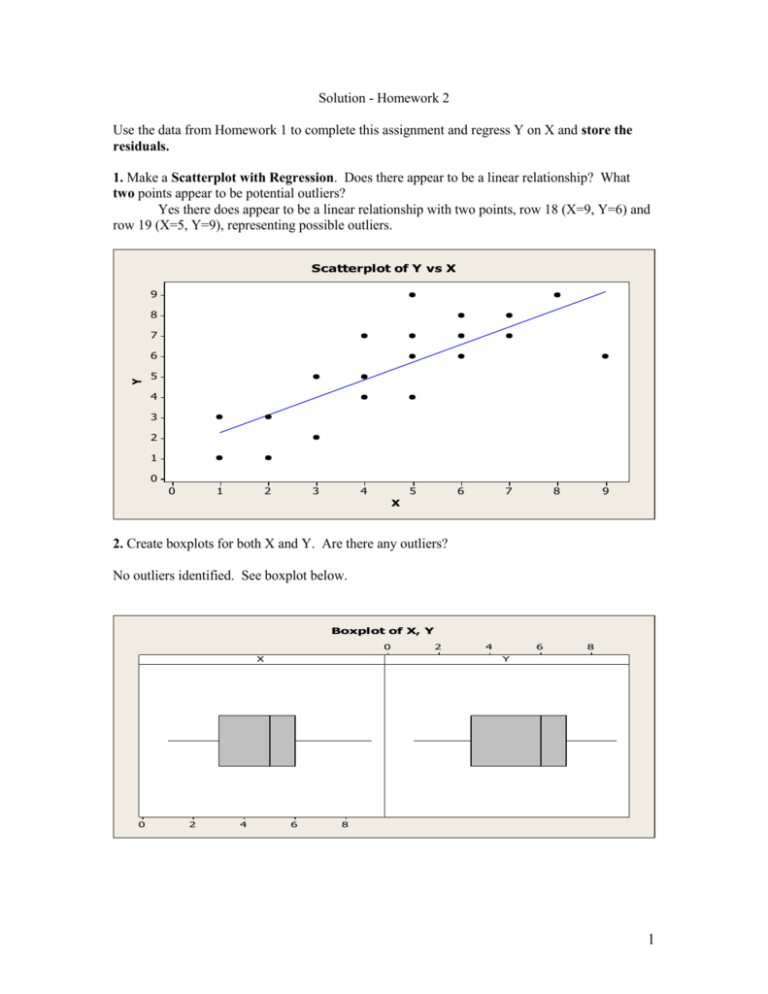
1. Make a Scatterplot with Regression. Does there appear to be a linear relationship? What
two points appear to be potential outliers?
Yes there does appear to be a linear relationship with two points, row 18 (X=9, Y=6) and
row 19 (X=5, Y=9), representing possible outliers.
Scatterplot of Y vs X
9
8
7
Y
6
5
4
3
2
1
0
0
1
2
3
4
5
6
7
8
9
X
2. Create boxplots for both X and Y. Are there any outliers?
No outliers identified. See boxplot below.
Boxplot of X, Y
0
X
0
2
4
2
4
6
8
Y
6
8
1
3. Do a check of normality by using a probability plot of the residuals. Include: a) the null and
alternative hypotheses, b) the p-value of the test, c) your decision based on a 0.05 level of
significance, and d) Minitab copy of your plot.
a) Ho: The residuals come from a normal distribution
Ha: The residuals do not come from a normal distribution
b) p-value is 0.942
c) Since p-value is greater than 0.05 we fail to reject Ho and will conclude the
assumption of normality is plausible.
d)
Probability Plot of RESI1
Normal - 95% CI
99
Mean
StDev
N
AD
P-Value
95
90
-2.13163E-15
1.556
20
0.158
0.942
Percent
80
70
60
50
40
30
20
10
5
1
-5.0
-2.5
0.0
RESI1
2.5
5.0
4. Do a check of equal variances by performing a Modified Levene Test. Include: a) the null and
alternative hypotheses, b) the p-value of the test, c) your decision based on a 0.05 level of
significance, and d) Minitab copy of your plot.
a) Ho: The variances are equal
Ha: The variances are not equal
b) The p-value is 0.533 NOTE: Remember that the Levene’s test is more robust against
violations to normality than is the F-test making the Levene test a better overall test of equal
variances. The only condition for the Levene test is that the variable being tested is continuous.
c) Since the p-value is greater than 0.05 we conclude that the assumption of equal
variances is plausible.
d)
2
Test for Equal Variances for RESI1
F-Test
Test Statistic
P-Value
0
0.83
0.861
group
Lev ene's Test
Test Statistic
P-Value
1
1.0
1.5
2.0
2.5
3.0
3.5
95% Bonferroni Confidence Intervals for StDevs
0.40
0.533
4.0
group
0
1
-4
-3
-2
-1
0
RESI1
1
2
3
5. Perform a Lack of Fit Test to check if linear regression function is appropriate. Include: a) the
null and alternative hypotheses, b) the correct F-statistic and p-value of the test, c) your decision
based on a 0.05 level of significance, and d) Minitab copy of your ANOVA output.
a) Ho: The linear regression function is appropriate
Ha: The linear regression function is not appropriate
b) F-statistic is 0.95 and p-value is 0.507
c) Since p-value is greater than 0.05 we fail to reject Ho and conclude plausible that
linear regression function is appropriate.
d)
Analysis of Variance
Source
Regression
Residual Error
Lack of Fit
Pure Error
Total
DF
1
18
7
11
19
SS
70.769
46.031
17.364
28.667
116.800
MS
70.769
2.557
2.481
2.606
F
27.67
P
0.000
0.95
0.507
6. Even though you may not have found any assumption violations perform a Box-Cox analysis
on Y to see if any transformation is suggested. Include the a) estimated and rounded lambda
values, b) the interpretation of this value, and c) the Box-Cox plot. NOTE: This can only be
done using Minitab Version 15 or higher – i.e. student version 14 does not contain Box-Cox
program.
a) Estimated value is 1.07 and rounded lambda is 1.00
b) The rounded value implies one raise Y to power of 1.00 which means no
transformation necessary
3
c)
Box-Cox Plot of Y
Lower C L
9
Upper C L
Lambda
StDev
(using 95.0% confidence)
8
Estimate
1.07
7
Lower C L
Upper C L
0.34
1.89
Rounded Value
1.00
6
5
4
3
Limit
2
-2
-1
0
1
2
Lambda
3
4
5
7. Find Bonferroni joint confidence intervals for Bo and B1 with a 90% family confidence level
and include your interpretation of these intervals. You can use the Minitab output to find s{bo}
and s{b1}
With sample size, n, of 20 the degrees of freedom are n-2 or 18. Since interested in two
joint intervals, Bo and B1, g is equal to 2 for our Bonferroni correction. Using the equations
bo  Bs{bo } and b1  Bs{b1} where B  t1n2/ 4 . From t-table the value for the Bonferrroni
multiplier using DF of 18 and 1-α/4 for alpha of 0.10 results in a 2.101 t-statistic. Plugging into
the equations:
For Bo: 1.377 +/- 2.101*0.8442 = 1.377 +/- 1.774 = -0.397 <= Bo <= 3.151
For B1: 0.8652 +/- 2.101*0.1645 = 0.8652 +/- 0.3456 = 0.5196 <= B1 <= 1.2108
Interpretation: We are 90% confident that both intervals contain the true intercept and slope.
8. Use Minitab to find Bonferroni simultaneous confidence intervals for new X observations of 0
and 10 using a 95% family confidence level. Include your the output and interpretation of these
intervals. Follow-up question 1: What is the interpretation of the level of confidence for the
confidence intervals in the output? Follow-up question 2: Can you think of a reason why these
new X values might not be reliable? Follow-up question 3: Show mathematically how one
would use the Minitab output to get the simultaneous level of confidence for new observations.
Interpretation: We are 95 percent confident in both of the following intervals being correct: that
the reading achievement stanine for a reading readiness stanine of 0 would be from -0.687 to
3.441 and the reading achievement stanine for a reading readiness stanine of 10 would be from
7.706 to 12.351
Predicted Values for New Observations
4
New
Obs
1
2
Fit
1.377
10.029
SE Fit
0.844
0.950
97.5% CI
(-0.687, 3.441)
( 7.706, 12.351)
97.5% PI
(-3.044, 5.798)
( 5.481, 14.576)X
X denotes a point that is an outlier in the predictors.
Values of Predictors for New Observations
New
Obs
1
2
X
0.0
10.0
Follow-up 1: The 97.5% level of confidence is how confident we are in any ONE of the intervals
being correct.
Follow-up 2: The range of x-values used in this analysis was from 1 to 9 bringing into
consideration the possibility of improper extrapolation of applying the regression equation to
values outside this range of x.
Follow-up 3: This 97.5% level of confidence is found using 1 – α/g = 0.975. For this particular
problem we are interested in two simultaneous intervals, or a g = 2. Using algebra to find alpha
we would get α/g = 0.025 resulting in 0.05 alpha or a 95% simultaneous level of confidence.
NOTE: Software systems by default use α/2 when constructing confidence intervals and is why
when solving this equation we do not use α/2 but instead α/g. If one were to use α/2g based on
the level of confidence in the output you would “double divide” by 2.
9. What is the value and interpretation of the coefficient of determination? Using the output and
correct values show two ways this value can be calculated.
From the output the coefficient of determination, or R-squared, is 60.6% meaning that 60.6
percent of the variation in reading achievement stanines can be explained by reading readiness
stanines.
S = 1.59914
R-Sq = 60.6%
R-Sq(adj) = 58.4%
Analysis of Variance
Source
Regression
Residual Error
Total
DF
1
18
19
SS
70.769
46.031
116.800
MS
70.769
2.557
F
27.67
P
0.000
Two possible methods for calculating R-squared are:
1) (SSR/SST)*100% = (70.769/116.8)*100% = 60.6%
2) [1 – (SSE/SST)]*100% = [1 – (46.031/116.8)]*100% = 60.6%
10. From our in class example of Sales-Advertising, the tests results were as follows: the
intercept had T = -0.16 and p-value of 0.885; the slope test had T = 3.66 and p-value of
0.035; and the ANOVA test had F = 13.66 and p-value of 0.035. Use Minitab to find this
5
p-values by going to Calc > Probability Distributions and selecting appropriately either T
or F. Then select the radio button for “Cumulative Probability”, enter the appropriate
degrees of freedom for the test, click the radio button for “Input Constant” and enter in
the text box the appropriate value of the test statistic. Click OK. From the output show
how one gets from this output to the p-value. Include a copy of the Minitab output for
each test.
Test of Intercept: From the output we would take 0.441524 and multiply by two to get
0.883 which is approximately 0.885 due to rounding.
Cumulative Distribution Function
Student's t distribution with 3 DF
x
-0.16
P( X <= x )
0.441524
Test of Slope: From output we would subtract 0.982377 from 1 and then double this
result getting 0.017623*2 = 0.035246 which is approximately 0.035
Cumulative Distribution Function
Student's t distribution with 3 DF
x
3.66
P( X <= x )
0.982377
F-Test: From this output we would simply subtract 0.96526 from 1 to get 0.03474 which
is approximately 0.035
Cumulative Distribution Function
F distribution with 1 DF in numerator and 3 DF in denominator
x
13.66
P( X <= x )
0.965626
NOTE: When using T, we need to double the result since the hypothesis test is 2-sided
and the T is symmetric. When our t-stat is negative we do not need to subtract from 1.
For the F-test this is already run as a 2-sided test so no need to double the result, but since
cumulative for a positive test statistic (which all F-statistics are) we must still subtract
from 1.
6