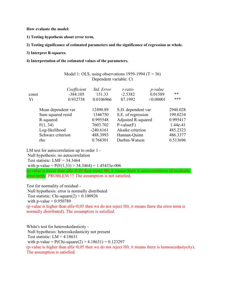
How evaluate the model:
1) Testing hypothesis about error term.
2) Testing significance of estimated parameters and the significance of regression as whole.
3) Interpret R-squares.
4) Interpretation of the estimated values of the parameters.
Model 1: OLS, using observations 1959-1994 (T = 36)
Dependent variable: Ct
const
Yt
Coefficient
-384.105
0.932738
Mean dependent var
Sum squared resid
R-squared
F(1, 34)
Log-likelihood
Schwarz criterion
rho
Std. Error
151.33
0.0106966
12490.89
1346750
0.995548
7603.702
-240.6161
488.3993
0.768301
t-ratio
-2.5382
87.1992
p-value
0.01589
<0.00001
S.D. dependent var
S.E. of regression
Adjusted R-squared
P-value(F)
Akaike criterion
Hannan-Quinn
Durbin-Watson
**
***
2940.028
199.0234
0.995417
1.44e-41
485.2323
486.3377
0.513696
LM test for autocorrelation up to order 1 Null hypothesis: no autocorrelation
Test statistic: LMF = 34.3464
with p-value = P(F(1,33) > 34.3464) = 1.45433e-006
(p-value is lower than alfa=0,05 then reject H0, it means there is autocorrelation of residualserror term) PROBLEM !!! The assumption is not satisfied.
Test for normality of residual Null hypothesis: error is normally distributed
Test statistic: Chi-square(2) = 0.100926
with p-value = 0.950789
(p-value is higher than alfa=0,05 then we do not reject H0, it means there the error term is
normally distributed). The assumption is satisfied.
White's test for heteroskedasticity Null hypothesis: heteroskedasticity not present
Test statistic: LM = 4.18631
with p-value = P(Chi-square(2) > 4.18631) = 0.123297
(p-value is higher than alfa=0,05 then we do not reject H0, it means there is homoscedastycity).
The assumption is satisfied.