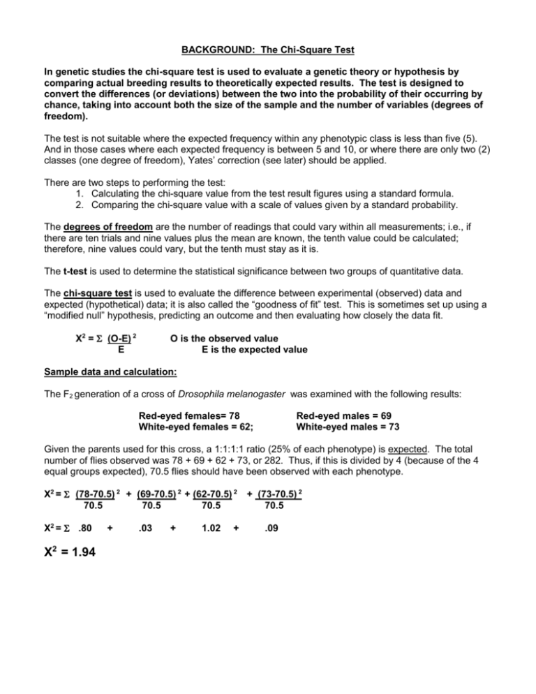
BACKGROUND: The Chi-Square Test
In genetic studies the chi-square test is used to evaluate a genetic theory or hypothesis by
comparing actual breeding results to theoretically expected results. The test is designed to
convert the differences (or deviations) between the two into the probability of their occurring by
chance, taking into account both the size of the sample and the number of variables (degrees of
freedom).
The test is not suitable where the expected frequency within any phenotypic class is less than five (5).
And in those cases where each expected frequency is between 5 and 10, or where there are only two (2)
classes (one degree of freedom), Yates’ correction (see later) should be applied.
There are two steps to performing the test:
1. Calculating the chi-square value from the test result figures using a standard formula.
2. Comparing the chi-square value with a scale of values given by a standard probability.
The degrees of freedom are the number of readings that could vary within all measurements; i.e., if
there are ten trials and nine values plus the mean are known, the tenth value could be calculated;
therefore, nine values could vary, but the tenth must stay as it is.
The t-test is used to determine the statistical significance between two groups of quantitative data.
The chi-square test is used to evaluate the difference between experimental (observed) data and
expected (hypothetical) data; it is also called the “goodness of fit” test. This is sometimes set up using a
“modified null” hypothesis, predicting an outcome and then evaluating how closely the data fit.
X2 =  (O-E) 2
E
O is the observed value
E is the expected value
Sample data and calculation:
The F2 generation of a cross of Drosophila melanogaster was examined with the following results:
Red-eyed females= 78
White-eyed females = 62;
Red-eyed males = 69
White-eyed males = 73
Given the parents used for this cross, a 1:1:1:1 ratio (25% of each phenotype) is expected. The total
number of flies observed was 78 + 69 + 62 + 73, or 282. Thus, if this is divided by 4 (because of the 4
equal groups expected), 70.5 flies should have been observed with each phenotype.
X2 =  (78-70.5) 2 + (69-70.5) 2 + (62-70.5) 2
70.5
70.5
70.5
X2 =  .80
X2 = 1.94
+
.03
+
1.02
+
+ (73-70.5) 2
70.5
.09
Students must next consult the Chi-Square table provided in the AP Biology laboratory manual to
determine whether or not this is within an acceptable range to support the hypothesis that the results are
due to the particular cross rather than a random change.
n
1
2
3
4
5
6
7
8
9
10
15
20
25
30
P= .99
.000157
.0201
.115
.297
.554
.872
1.239
1.646
2.088
2.558
5.229
8.260
11.524
14.953
P =.95
.00393
.103
.352
.711
1.145
1.635
2.167
2.733
3.325
3.940
7.261
10.851
14.611
18.493
P = .80
.0642
.446
1.005
1.649
2.343
3.070
3.822
4.594
5.380
6.179
10.307
14.578
18.940
23.364
P = .50
.455
1.386
2.366
3.357
4.351
5.348
6.346
7.344
8.343
9.342
14.339
19.337
24.337
29.336
P = .20
1.642
3.219
4.642
5.989
7.289
8.558
9.803
11.030
12.242
13.442
19.311
25.038
30.675
36.250
P = .05
3.841
5.991
7.815
9.488
11.070
12.592
14.067
15.057
16.919
18.307
24.996
31.410
37.652
43.773
P = .01
6.635
9.210
11.345
13.277
15.086
16.812
18.475
20.090
21.666
23.209
30.578
37.566
44.314
50.892
An estimation of the probability value is obtained by looking along the line representing the number of
phenotypic classes being considered and comparing the calculated chi-square value to those in the table
(degrees of freedom = n = # of actual phenotypic classes – 1). The calculated value will lie between two
values corresponding to percentages at the head of the table.
Obtaining a precise value is not the purpose of this test. What is important is to determine whether
the deviations from theoretically expected results are of such significance as to invalidate the
theory being examined. The significant level is customarily set at 5% so that, for instance, where there
are two phenotypic classes (degrees of freedom, n = 1), the figure of 3.84 marks the division between
deviations which are significant and those which are not significant.
**Using the sample data, for 4 phenotypic classes (n = 3), a chi-square value of 1.94 is obtained which
lies between values indicating probabilities of 50% and 80%; let’s say 60%. This indicates that in a large
number of similar tests deviations as great as, or greater than that observed, would occur in about 60%
of those tests by chance alone. This is greater than the significant 5% level and we can conclude that
this test does NOT invalidate theoretical expectations.
Now you try!…
Problem: Using Mendel’s methods in crossing pea plants, the following results were collected in a cross
between two plants heterozygous for seed shape and seed color (RrYy X RrYy).
(R = round, r = wrinkled; Y = yellow, y = green)
RESULTS: 547 yellow-round; 193 green-round; 195 yellow-wrinkled; 65 green-wrinkled.
a) What are the expected phenotype ratios in the offspring?
b) In 1000 offspring, how many are expected of each phenotype?
c) Perform a Chi-Square test with the results obtained. Do these results invalidate theoretical
expectations?