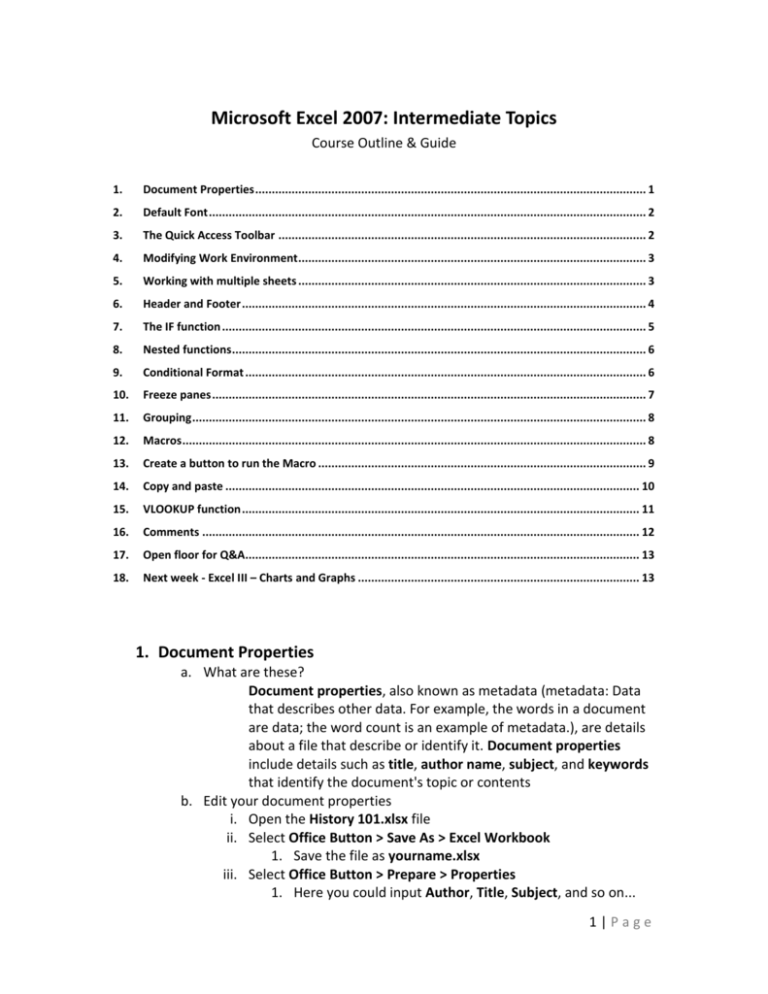
Microsoft Excel 2007: Intermediate Topics
Course Outline & Guide
1.
Document Properties ...................................................................................................................... 1
2.
Default Font .................................................................................................................................... 2
3.
The Quick Access Toolbar ............................................................................................................... 2
4.
Modifying Work Environment ......................................................................................................... 3
5.
Working with multiple sheets ......................................................................................................... 3
6.
Header and Footer .......................................................................................................................... 4
7.
The IF function ................................................................................................................................ 5
8.
Nested functions ............................................................................................................................. 6
9.
Conditional Format ......................................................................................................................... 6
10.
Freeze panes ................................................................................................................................... 7
11.
Grouping ......................................................................................................................................... 8
12.
Macros ............................................................................................................................................ 8
13.
Create a button to run the Macro ................................................................................................... 9
14.
Copy and paste ............................................................................................................................. 10
15.
VLOOKUP function ........................................................................................................................ 11
16.
Comments .................................................................................................................................... 12
17.
Open floor for Q&A....................................................................................................................... 13
18.
Next week - Excel III – Charts and Graphs ..................................................................................... 13
1. Document Properties
a. What are these?
Document properties, also known as metadata (metadata: Data
that describes other data. For example, the words in a document
are data; the word count is an example of metadata.), are details
about a file that describe or identify it. Document properties
include details such as title, author name, subject, and keywords
that identify the document's topic or contents
b. Edit your document properties
i. Open the History 101.xlsx file
ii. Select Office Button > Save As > Excel Workbook
1. Save the file as yourname.xlsx
iii. Select Office Button > Prepare > Properties
1. Here you could input Author, Title, Subject, and so on...
1|Page
2. This information will stay with the workbook until changed
3. Select the X to the far right of the Document Properties
window panel
2. Default Font
a. What is this?
A typeface instruction that a computer assumes for Word, which
is typically Times New Roman. A user may change this typeface in
Word to be different the next time Word is opened
b. Set your new default font
i. Select Office Button > Excel Options (button in bottom right of
window) >Popular > When creating new workbooks
1. Click a font in the Use this font box, and then specify a
font size in the Font Size box
2. In order to begin using the new default font and font size,
you must restart Excel. The new default font and font size
are used only in new workbooks that you create after you
restart Excel; existing workbooks are not affected
3. The Quick Access Toolbar
a. What is this?
The Quick Access Toolbar is a customizable toolbar containing a
set of commands
b. The toolbar is located in the top left-hand corner of the window, just to
the right of the Office button
c. To customize your Quick Access Toolbar, move your mouse pointer to
the far right of the toolbar and select the down arrow
i. Customize Quick Access Toolbar
1. You can add or remove commands/shortcuts from the
toolbar here
2. Add any command/shortcut
a. At the bottom of the window select, More
Commands…
b. In the Choose commands from… text box, select a
group, and then select a command/shortcut from
the list below
c. Select the Add button to move it to the column to
the right, and then select the OK button
3. An easier approach is to locate the tool on the Ribbon,
right-click on that command/shortcut, and select to Add to
Quick Access Toolbar from the menu
2|Page
4. Modifying Work Environment
a. What is this?
This section primarily covers how you can set your preferences for
specific view, display, and editing settings in the Options dialog
box (Tools menu, Options command)
b. Select Office Button > Excel Options
i. Popular
1. Hover your mouse pointer on the check box to view
information on each one
a. Show Mini Toolbar…, Enable Live Preview, and so
on...
2. Personalize your copy of Microsoft Office
a. User Name is used when creating a new workbook
ii. Saving
1. Save workbooks
a. Check the box next to Save AutoRecover
information every so Excel will automatically save
your workbook every so many minutes in the event
that Excel is closed unexpectedly. Every 10 minutes
is a recommended setting
b. Default file location: changes the place you want
to save most of you workbooks
iii. Advanced
1. There are many options that you can change and should
be aware of as you use Excel
2. Editing options
a. The are many useful options here, like After
pressing Enter, move selection Direction …so look
them over briefly for now, but it would be a wise
decision to look these over again after class
3. Display
a. Show formula bar
i. Extremely useful and one that should
always be checked
b. For cells with comments, show:
i. Indicators only, and comments on hover
should be selected as it is the easiest to
work with
5. Working with multiple sheets
a. What are these?
3|Page
The primary documents that you use in Excel to store and work
with data. A worksheet consists of cells that are organized into
columns and rows; a worksheet is always stored in a workbook
b. Multiple worksheets
i. To access a worksheet
1. Click on the tab in the bottom left corner of the named
Sheet 1, Sheet 2, or Sheet 3
a. Each sheet opens once selected
b. As a default, you begin with 3 worksheets
ii. To rename a worksheet
1. Move your mouse pointer inside the Sheet 1 tab and rightclick
a. A menu will appear with options including Insert...,
Rename, Delete, and so on
b. Select Rename
c. Type, Grade Sheet
d. Tap the Enter key
6. Header and Footer
a. What are these?
These are optional areas for text like page numbers, author name,
and title that are repeated at the top and bottom of the page. The
space provided for these does not affect the space for the main
content of the page
b. Begin from the top of the worksheet
i. Use the Ctrl+Home keyboard shortcut
c. Edit the header
i. On the Ribbon, select the View tab > in the Workbook Views
group > click Page Layout
1. You should now see the header and footer sections at the
top and bottom of the page
ii. Insert data in header
iii. Note: the Ribbon now has a new contextual tab named Design
under Header & Footer Tools and you are currently working with
this tab while editing your header
1. Click inside the first of three boxes in the header
a. Type, Fall 2007
2. Click inside the second of three boxes in the header
a. On the Ribbon, select the Design tab > in the
Header & Footer Elements group > click Sheet
Name
b. You will now see &[Tab] in the box
4|Page
iv. Click once inside the main body of the document when finished
editing the header
d. Edit the footer
i. While still in Page Layout
ii. Insert data in footer
1. Click inside the first of three boxes in the footer
2. Insert Current Date
a. On the Ribbon, select the Design tab > in the
Header & Footer Elements group > click Current
Date
b. You will now see &[Date] in the box
3. Insert Page Number
4. Click inside the third of three boxes in the footer
a. On the Ribbon, select the Design tab > in the
Header & Footer Elements group > click Page
Number
b. You will now see &[Page] in the box
iii. Click once inside the main body of the document when finished
editing the header
e. On the Ribbon, select the View tab > in the Workbook Views group >
click Normal
7. The IF function
a. What is this?
A function that returns one value if a condition you specify
evaluates to TRUE and another value if it evaluates to FALSE. Use
IF to conduct conditional tests on values and formulas
b. Use the IF function
i. Create a new field
1. Select cell I3
2. Type, Pass/Fail
3. Tap the Enter key
ii. Select the IF function
1. With cell I4 now selected…
2. On the Ribbon, select the Formulas tab > in the Function
Library group > click Logical > IF
3. You are now working with this function:
a. =IF(logical_test,value_if_true,value_if_false)
i. Logical_test: type, H4>=70
ii. Value_if_true: type, Pass
iii. Value_if_false: type, Fail
b. Click the OK button (bottom right)
4. Result should be, Pass
5|Page
c. Carry the function down for the other students
i. Select cell I4
ii. Use the Fill Handle and drag from cell I4 to cell I7
d. Test the cell reference of the IF function
i. Select Sierra’s Quiz 3 (cell D6)
ii. Change her grade from 88 to 0
iii. Notice how Sierra changes from passing the class to failing
iv. Change her quiz grade back from 0 to 88
e. Continue to input data into the Grade Sheet worksheet
i. In cell J3 type:
1. Letter Grade
2. Tap the Enter key
8. Nested functions
a. What is this?
Nested functions use a function as one of the arguments of
another function. You can nest up to 64 levels of functions
b. Nest the IF function
i. Select cell J4
ii. Click inside the Formula Bar
iii. Type:
1. =IF(H4>=90,"A",
iv. When you have more than 1 possible False outcome value, then
you should nest an IF function in the False section. If you
have only 1 False value remaining, then simply input the
False value and do not nest another IF function
c. Challenge the class to complete =IF(H4>=90,"A", for letter grades:
i. A, B, C, D, F
ii. The final nested IF function should be:
=IF(H4>=90,"A",IF(H4>=80,"B",IF(H4>=70,"C",IF(H4>=60,"D","F"))))
d. Carry the function down for the other students
i. Select cell J4
ii. Use the Fill Handle and drag from cell J4 to cell J7
e. Test the cell reference of the nested IF function
i. Select Sierra’s Quiz 3 (cell D6)
ii. Change her grade from 88 to 0
iii. Notice how Sierra’s changes from passing the class to failing and
that her name letter grade is a D
iv. Change her quiz grade back from 0 to 88
9. Conditional Format
a. What is this?
6|Page
A format, such as cell shading or font color, that Excel
automatically applies to cells if a specified condition is true
b. Apple a conditional format
i. Select cells I4 to I7 (the students Pass/Fail value cells)
ii. On the Ribbon, select the Home tab > in the Styles group > click
Conditional Formatting > New Rule...
iii. In the New Formatting Rule window, under select a rule type:
1. Different rule descriptions will appear below when
selecting a different type
2. Choose Format only cells that contain
3. Below, in Edit the rule description
a. Format only cells with:
i. Cell value, equal to, and type in Pass
b. Click on the Format button
i. In the new Format Cells window click on
the Fill tab
ii. Choose a light blue color
iii. Click the OK button
iv. The color of the cells with the value Pass are now blue
c. Create an additional conditional format
i. Select cells I4 to I7
ii. On the Ribbon, select the Home tab > in the Styles group > click
Conditional Formatting > Manage Rules...
iii. In the Conditional Formatting Rules Manager window
1. Click the New Rule... button
a. Just as before, create a new rule, but this time for
the value Fail and use a fill color of red with a white
colored white
b. Click the OK button
2. You now should have two conditional format rules
3. Click the OK button
10. Freeze panes
a. What is this?
A pane is a portion of the document window bounded by and
separated from other portions by vertical or horizontal bars.
These panes can be “frozen” essentially locking the columns and
rows
b. Freeze the students names and the field names
i. Select cell B4
ii. On the Ribbon, select the View tab > in the Window group > click
Freeze Panes > Freeze Panes (in drop down menu)
c. Demonstrate how this works
7|Page
i. Using the worksheet scrollbar, show how the column and rows
are locked (frozen)
d. Unlock panes
i. On the Ribbon, select the View tab > in the Window group > click
Freeze Panes > Unfreeze Panes (in drop down menu)
11. Grouping
a. What is this?
Columns and/or rows can be grouped together where they are
treated as one object. In grouping them you gain the ability to
“open” or “close”, “show” or “hide” the group. It is especially
beneficial when you are working with large amounts of data that
have defined “groups” and/or if you want to print some of the
data, but not all
b. Group columns together
i. On the Ribbon, select the Data tab > in the Outline group > click
Group > Group... (in drop down menu)
ii. Above the column letter ID’s you should now see a line with a –
(minus) sign to the right
1. Click on this line to “hide” the group
2. Click on the + (plus) sign to “show” the group
iii. Printing
1. Try “hiding” the group and go to Print Preview
2. What is “hidden” will not print
12. Macros
a. What is this?
An action or a set of actions that you can use to automate tasks.
Macros are recorded in the Visual Basic for Applications
programming language
b. Create a macro
i. If the Developer tab is not available, do the following to display it:
1. Select Office Button > Excel Options button
2. In the Popular category, under Top options for working
with Excel, select the Show Developer tab in the Ribbon
check box, and then click OK
3. You now have a new Ribbon tab named, Developer
ii. Record a macro
1. On the Developer tab, in the Code group, click Record
Macro
a. In the Macro name: text box type:
GradesAscending
8|Page
i. Note: the first character of the macro name
must be a letter. Following characters can
be letters, numbers, or underscore
characters. Spaces are not allowed in a
macro name; an underscore character
works well as a word separator. If you use a
macro name that is also a cell reference,
you may get an error message that the
macro name is not valid.
b. Describe the shortcut key
i. The shortcut key will override any
equivalent default Excel shortcut key while
the workbook that contains the macro is
open
c. Store Macro In: This Workbook
d. Description: Sort the grades in ascending order
e. Click the OK button
2. Perform the action you want to record
a. Select the cells A3 to J7
b. Right click inside the selected cells
c. From the menu, select Sort > Custom Sort...
d. Under Column, in the box next to Sort By choose
Final Grade
e. Under Sort On, choose Values
f. Under Order, choose Smallest to Largest
g. Click the OK button
3. Stop the recording
a. On the Developer tab, in the Code group, click Stop
Recording
b. Your new macro is now available to be run at any
time
13. Create a button to run the Macro
a.
What is this?
Shapes can be created to be used as a button. To turn a shape
into a button you can create a hotspot which is a linkable shape
area
b. Create a shape
i. On the Insert tab, in the Illustrations group, click Shapes drop
down menu arrow), under Rectangles, click Rounded Rectangle
ii. Move your mouse pointer into a empty are inside your worksheet,
click and drag out a rounded rectangle
c. Create a hotspot by assigning a macro
9|Page
d.
e.
f.
g.
i. Right click inside the shape and from the menu click Assign
Macro...
1. Select GradesAscending
2. Select the OK button
Sort the students in descending order
i. Select the cells A3 to J7
ii. Right click inside the selected cells
iii. From the menu, select Sort > Custom Sort...
iv. Under Column, in the box next to Sort By choose Final Grade
v. Under Sort On, choose Values
vi. Under Order, choose Largest to Smallest
vii. Click the OK button
Use your new button to run the macro
i. Click once on the rounded rectangle shape (button) you created
ii. Notice how the students are now sorted in ascending order
Continue to work in the workbook
i. Right click on the Sheet 2 tab in the bottom left-hand corner
ii. From the menu select: Rename
1. Call the Sheet: Financial Aid
Save a Macro enabled workbook
i. A way to preserve the file by keeping the macros you created
ii. Select Office Button > Save As (arrow to the right) > MacroEnabled Workbook
iii. Save the file using the same name, but choose the .xlsm file
format
iv. You must save in this file format to keep the macros working
14. Copy and paste
a. What is this?
In Excel you can copy text, images, functions, and much more in
order to paste (put) it into another location. You can copy and
paste within one worksheet or from one to another
b. Copy an item
i. Select the cells from A4 to A7
ii. On your keyboard, use the keyboard shortcut Ctrl+C
c. Paste and item
i. Select the Financial Aid worksheet
ii. Select cell A1
iii. On your keyboard, use the keyboard shortcut Ctrl+V
iv. At this point in time, if you change the data in the Grade Sheet
then the data does not change in the Financial Aid sheet
d. Copy and Paste Special
i. Copy
10 | P a g e
1. Select the Grade Sheet worksheet
2. Select the cells from A4 to A7
3. On your keyboard, use the keyboard shortcut Ctrl+C
ii. Paste Special
1. Select the Financial Aid sheet
2. Select cell A1
3. On the Ribbon, select the Home tab > in the Clipboard
group > click Paste (drop down arrow) > Paste Special...
4. Paste Special is a very useful option as you could paste
specific parts of the item you have just copied
5. Click on Cancel
e. Paste Link
i. On the Ribbon, select the Home tab > in the Clipboard group >
click Paste (drop down arrow) > Paste Link
1. The items appear as they would if pasted normally, but
now Excel uses a cell reference to display the information
2. Select any cell that has an item just pasted, and the look
inside the formula bar
3. This creates an environment conducive for worksheet
flow, where items that are changes flow from one sheet
into the next
4. In Grade Sheet, change Tiffany’s name to Rachelle
5. Select the Financial Aid sheet and notice that Tiffany’s
name is now Rachelle
15. VLOOKUP function
a. What is this?
Searches for a value in the first column of a table array and
returns a value in the same row from another column in the table
array.
The V in VLOOKUP stands for vertical. Use VLOOKUP instead of
HLOOKUP when your comparison values are located in a column
to the left of the data that you want to find.
b. Use the VLOOKUP function
i. Setup Lookup input/output area
1. Rename Sheet 3 to View Grades
2. In cell A1 type, View Student Grades
3. In cell A3 type, Student
4. In cell A4 type, Final Grade
5. In cell A5 type, Letter Grade
ii. Create a VLOOKUP function
1. Select cell B4
11 | P a g e
2. On the Ribbon, select the Formulas tab > in the Function
Library group > click Lookup & Reference (drop down
arrow) > VLOOKUP
3. In the Function Arguments window
a. Click inside the box to the right of Lookup_value
b. In the Financial Aid sheet select cell B3
c. Click inside the box to the right of Table_array
d. Select the Grade Sheet worksheet
e. Select cells A4 to J7
i. You should see 'Grade Sheet'!A4:J7 in the
box
f. Click inside the Col_index_num box and type 8
i. This will return the value in the 8th row of
the table array
g. Note: the table array’s ID or Lookup Value must be
sorted in ascending order to work
h. Click OK
i. The Formula bar should now display
=VLOOKUP(B3,'Grade Sheet'!A4:J7,8)
4. Lookup a value
a. Select cell B3 and type John
b. The Vlookup will not work because the names are
not sorted
iii. Challenge the class to create a macro in the View Grades sheet to
sort the names in ascending order so you can successfully run the
Vlookup
1. After giving time for the students in the class to finish, go
over the process of the class challenge
iv. Challenge the class to create another Vlookup for the students
Letter Grade
v.
After giving time for the students in the class to finish, go
over the process of the class challenge
16. Comments
a. What are these?
In Microsoft Office Excel, you can add a note to a cell by inserting
a comment. You can edit the text in comments and delete
comments that you no longer need.
b. Insert a comment
i. Select cell J7 (Sierra’s letter grade)
ii. On the Ribbon, select the Review tab > in the Comments group >
click New Comment
12 | P a g e
iii. In the comment note window type, Sierra is working on extra
credit. Do not post grade until 12/20/2007
iv. Tap the Enter key
c. Comment Options
i. You can edit a comment, navigate from one comment to the
next, and show/hide comments for printing.
17.Open floor for Q&A
18. Next week - Excel III – Charts and Graphs
a. TBD…
13 | P a g e