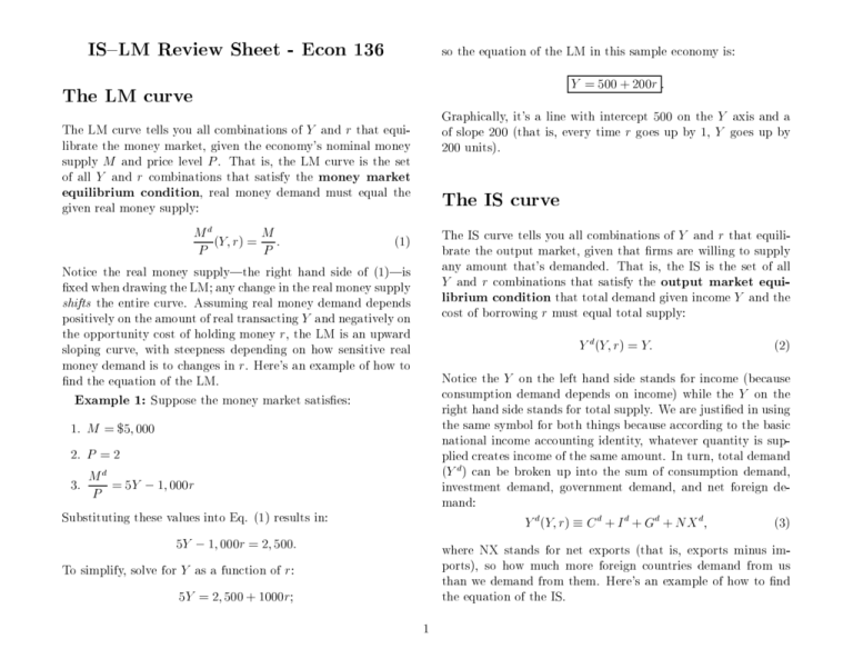
so the equation of the LM in this sample economy is:
IS{LM Review Sheet - Econ 136
Y
The LM curve
Graphically, it's a line with intercept 500 on the Y axis and a
of slope 200 (that is, every time r goes up by 1, Y goes up by
200 units).
The LM curve tells you all combinations of Y and r that equilibrate the money market, given the economy's nominal money
supply M and price level P . That is, the LM curve is the set
of all Y and r combinations that satisfy the money market
equilibrium condition, real money demand must equal the
given real money supply:
M
P
d
(Y; r) =
M
P
:
The IS curve
The IS curve tells you all combinations of Y and r that equilibrate the output market, given that rms are willing to supply
any amount that's demanded. That is, the IS is the set of all
Y and r combinations that satisfy the output market equilibrium condition that total demand given income Y and the
cost of borrowing r must equal total supply:
(1)
Notice the real money supply|the right hand side of (1)|is
xed when drawing the LM; any change in the real money supply
shifts the entire curve. Assuming real money demand depends
positively on the amount of real transacting Y and negatively on
the opportunity cost of holding money r, the LM is an upward
sloping curve, with steepness depending on how sensitive real
money demand is to changes in r. Here's an example of how to
nd the equation of the LM.
Example 1: Suppose the money market satises:
1.
M
2.
P
3.
Y
=2
P
d
= 5Y
1; 000r
Substituting these values into Eq. (1) results in:
5Y
d
(Y; r) = Y:
(2)
Notice the Y on the left hand side stands for income (because
consumption demand depends on income) while the Y on the
right hand side stands for total supply. We are justied in using
the same symbol for both things because according to the basic
national income accounting identity, whatever quantity is supplied creates income of the same amount. In turn, total demand
(Y d ) can be broken up into the sum of consumption demand,
investment demand, government demand, and net foreign demand:
d
d
d
d
d
Y (Y; r ) C + I + G + N X ;
(3)
= $5; 000
M
= 500 + 200r :
1; 000r = 2; 500:
where NX stands for net exports (that is, exports minus imports), so how much more foreign countries demand from us
than we demand from them. Here's an example of how to nd
the equation of the IS.
To simplify, solve for Y as a function of r:
5Y = 2; 500 + 1000r;
1
Suppose the output market satises:
Example 2:
d
1.
C
2.
I
3.
G
4.
NX
d
d
= 1000 + :5(Y
= 500
T
), where
T
r
IS
= 600
100r
LM
8.75
= 600
d
= 200
500
Notice consumption demand depends on after tax income Y T
and investment demand depends on the cost of borrowing r,
that's why total demand (Y d ) depends on both Y and r. Adding
the 4 components of total demand together after substituting in
the value of T we nd total demand is:
Y
d
= [700 + :5Y ] + [500
d
100r] + 600 + 200;
= 2; 000 + :5Y
4,000
Y
Putting it together, in our sample economy the IS and LM
curves look like the above. They intersect at Y = 2; 250 and
1
r = 8:75. [Of course this is a very unrealistic interest rate since
8.75 = 875%!] This is the short run (SR) equilibrium of the
economy: where both the money market and the output market
are in equilibrium. A SR equilibrium also is a long run (LR)
equilibrium if there is full employment, i.e., if the labor market
also is in equilibrium. In particular, the above SR equilibrium
also is a LR equilibrium if and only if there is enough demand for
full employment, i.e., if and only if 2; 250 is the full employment
output level Y FE .
which simplies to
Y
2,250
100r:
Now use the output market equilibrium condition, Eq. (2)
above, to nd the IS. If rms will supply whatever is demanded,
then
2; 000 + :5Y 100r = Y:
To simplify, solve for Y as a function of r:
5 = 2; 000
: Y
100r;
so the equation of the IS curve in this sample economy is
Y
= 4; 000
1 To
nd the crossing place, you need to nd where Y = 500 + 200r (on
the LM) and Y = 4000 200r (on the IS). Solving these 2 equations in 2
unknowns, i.e., putting the 2 together, we see that at the crossing place:
200r :
500 + 200r = 4000
Graphically, it's a line with intercept of 4,000 on the Y axis and
a slope of -200 (that is, every time r increases by 1, Y goes down
by 200 units).
200r;
hence r = 8:75. Plugging this value for r into either the IS or LM equation
shows Y = 2250.
2