ECON 222
Macroeconomic Theory I
Fall Term 2010
Assignment 4
Due: Drop Box 2nd Floor Dunning Hall by noon November 26th 2010
No late submissions will be accepted
No group submissions will be accepted
No “Photocopy” answers will be accepted
Remarks: Write clearly and concisely. Present graphs, plots and tables in a format that is easy to understand.
The way you present your answers will be reflected in the final grade. Even if a question is mainly analytical,
briefly explain what you are doing, stressing the economic meaning of the various steps.
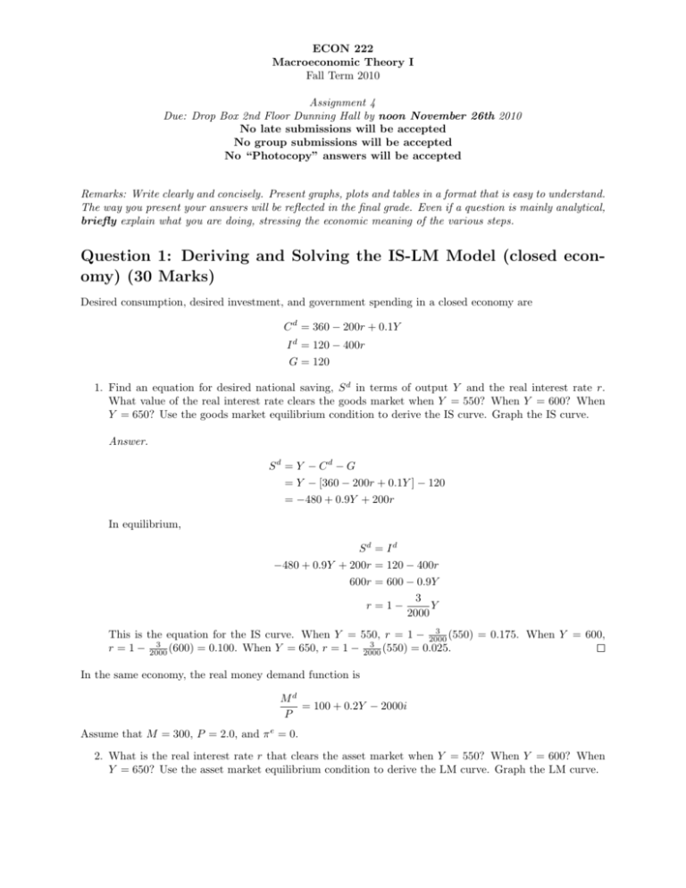
Question 1: Deriving and Solving the IS-LM Model (closed economy) (30 Marks)
Desired consumption, desired investment, and government spending in a closed economy are
C d = 360 − 200r + 0.1Y
I d = 120 − 400r
G = 120
1. Find an equation for desired national saving, S d in terms of output Y and the real interest rate r.
What value of the real interest rate clears the goods market when Y = 550? When Y = 600? When
Y = 650? Use the goods market equilibrium condition to derive the IS curve. Graph the IS curve.
Answer.
Sd = Y − Cd − G
= Y − [360 − 200r + 0.1Y ] − 120
= −480 + 0.9Y + 200r
In equilibrium,
Sd = I d
−480 + 0.9Y + 200r = 120 − 400r
600r = 600 − 0.9Y
3
Y
r =1−
2000
3
This is the equation for the IS curve. When Y = 550, r = 1 − 2000
(550) = 0.175. When Y = 600,
3
3
r = 1 − 2000 (600) = 0.100. When Y = 650, r = 1 − 2000 (550) = 0.025.
In the same economy, the real money demand function is
Md
= 100 + 0.2Y − 2000i
P
Assume that M = 300, P = 2.0, and π e = 0.
2. What is the real interest rate r that clears the asset market when Y = 550? When Y = 600? When
Y = 650? Use the asset market equilibrium condition to derive the LM curve. Graph the LM curve.
Answer. The asset market equilibrium condition is
Md
M
= 100 + 0.2Y − 2000(r + π e ) =
P
P
(1)
Substituting the values for M , P , and π e yields the equation for the LM curve:
300
2
2000r = −50 + 0.2Y
1
Y
r=− +
40 10000
100 + 0.2Y − 2000r =
When Y = 550, r = −1/40 + (550)/10000 = 0.030. When Y = 600, r = −1/40 + (600)/10000 = 0.035.
When Y = 650, r = −1/40 + (650)/10000 = 0.04.
Now suppose that the full employment level of output is Ȳ = 640. Add the FE line to your graph with the
IS and LM curves. If there is no point where all three curves intersect, the economy must not be in general
equilibrium. One of the assumptions of the IS-LM framework is that the price level P adjusts to restore
general equilibrium.
3. To what price level P does the economy converge in order to restore general equilibrium in this
economy? During this time of price level adjustment, by how much does the actual rate of inflation
exceed the expected rate of inflation, π e = 0?
Answer. In the goods market, the equilibrium interest rate when output is at its full employment level
is
3
(640) = 0.040
r =1−
2000
Now for the asset market equilibrium condition to hold, we can substitute the full employment level of
output Ȳ = 640 and the equilibrium interest rate r = 0.040 and solve for the price level P .
Md
M
= 100 + 0.2Y − 2000(r + π e ) =
P
P
300
100 + 0.2(640) − 2000(0.04) =
P
300
P =
≈ 2.0270
148
During the period of adjustment toward general equilibrium, expected inflation was π e = 0 but the
price level actually rose by 1.35% (π = (2.027 − 2)/2). Therefore, the actual rate of inflation exceeded
the expected rate of inflation by 1.35%.
Question 2: Shocking to the IS-LM Model (closed economy) (25
marks)
Consider the following economy:
C d = 200 + 0.5Y − 500r
I d = 200 − 500r
L = 0.5Y − 250(r + π e )
πe = 0
G = 150
M = 4900
Ȳ = 1000
2
r
F E(3)
LM(3)
LM(2)
r(3) = 0.04
IS(1)
Y
Ȳ = 640
Figure 1: Question 1
1. What are the general equilibrium levels of the real interest rate r, the price level P , desired aggregate
consumption C d , and desired investment I d ?
Answer. The IS curve:
Sd = I d
Y − Cd − G = Id
Y − [200 + 0.5Y − 500r] − 150 = 200 − 500r
Y
⇒ r = 0.55 −
2000
The intersection with the FE line yields a general equilibrium interest rate of r = 0.55 − 1000
2000 = 0.05.
At output equal to Ȳ and with the equilibrium interest rate calculated above, the general equilibrium
levels of consumption and investment are
C d = 200 + 0.5(1000) − 500(0.05) = 675
I d = 200 − 500(0.05) = 175
Finally, the price level will adjust in the asset market until the LM curve intersects at the same point,
(r = 0.05, Y = 1000). The LM curve is given by
M
= L = 0.5Y − 250(r + π e )
P
Substituting M = 4900, π e = 0, and the general equilibrium values of Y and r, we can solve for the
general equilibrium price level:
4900
= 0.5(1000) − 250(0.05 + 0)
P
⇒ P = 10.05
2. Suppose that the majority of economic activity in this economy is wine-making. Because vineyards are
highly sensitive to the climate, let’s imagine that the weather this year is unusually conducive to growing
3
grapes. In the IS-LM framework, this situation represents a beneficial supply shock. Specifically,
suppose the full-employment level of output Ȳ increases temporarily to Ȳ 0 = 1050. Show what happens
to the economy in a graph. What will be the new long-run equilibrium value of r and how will the
new general equilibrium come about? What is the new price level P ?
Answer. The beneficial supply shock shifts the FE line up to Ȳ 0 . The new equilibrium point is at the
intersection of the FE’ line and the IS curve. The economy is no longer in general equilibrium because
there is no point on the graph where all three curves intersect. In the long-run, the price level adjusts
downward to shift the LM curve down and to the right, until it passes through the new equilibrium
point.
We can solve for the new equilibrium point by finding the intersection of the IS curve and the FE’ line:
r = 0.55 −
Y
1050
= 0.55 −
= 0.025
2000
2000
Finally, the price level will adjust in the asset market until the LM curve intersects at the same point,
(r = 0.025, Y = 1050). Using LM curve, we can solve for the general equilibrium price level:
4900
= 0.5(1050) − 250(0.025 + 0)
P
⇒ P = 9.446
3. Consider again the positive supply shock from part 2. The Bank of Canada does not want the price
level to fall. To prevent this from happening, the Bank of Canada conducts open market operations
to adjust the supply of money in the economy, M . By how much does the money supply M have to
change in order to prevent the price level from changing? Does this involve an open market purchase
or an open market sale?
Answer. Instead of allowing the price level to adjust, we’ll shift the LM curve by changing the nominal
money supply, M :
M
= 0.5(1050) − 250(0.025)
10
⇒ M = 5187.5
Therefore, the Bank of Canada has to increase the money supply from 4900 to 5187.5, which involves an
open market purchase. Specifically, the Bank must buy government bonds with newly minted currency
in order to increase the stock of money in the economy.
Question 3: Deriving the AD Curve (closed economy) (20 marks)
Consider an economy with the following IS and LM curves:
Y = 4350 − 800r + 2G − T
M
= 0.5Y − 200r
P
(IS)
(LM)
1. Suppose that T = G = 450 and that M = 9000. Find an equation for the aggregate demand curve.
[Hint: Use the IS and LM equations to find a relationship between Y and P ]. If the full-employment
level of output is Ȳ = 4600, what are the equilibrium values for r and P ? Illustrate the long-run
equilibrium in the AD-AS diagram.
4
r
F E F E0
LM
LM 0
IS
Ȳ = 1000
Ȳ 0 = 1050
Y
Figure 2: Question 2, part 2
Answer. Substituting T = G = 450 and M = 9000 into the IS and LM equations gives
4800
Y
−
800
800
9000
18000
Y
= 0.5Y − 200r ⇒ r = −
+
P
400P
400
Y = 4350 − 800r + 2(450) − 450 ⇒ r =
Since both the IS and LM equations give expressions for r, we can eliminate r by setting them equal
to each other:
Y
18000
Y
4800
−
=−
+
800
800
400P
400
4800
3Y
36000
−
=−
800
800
800P
12000
⇒ Y = 1600 +
P
This is the AD equation. At Ȳ = 4600, solving for the price level yields P = 4. Using the IS curve (or
alternatively the LM curve with Y = 4600 and P = 4), we can solve for the equilibrium interest rate,
r = 0.25.
2. Repeat part 1 for T = G = 330 and M = 9000 with Ȳ fixed. Repeat part 1 for T = G = 450 and
M = 4500 with Ȳ fixed. You don’t have to draw more AD-AS graphs.
Answer. Following the same steps as above with T = G = 330 instead of 450, the AD curve is
Y = 1560 +
12000
.
P
At Ȳ = 4600, this gives P = 3.947. From the IS or LM curve, the equilibrium real interest rate is
r = 0.10.
Following the same steps as above with M = 4500 instead of 9000, the AD curve is
Y = 1600 +
5
6000
.
P
At Ȳ = 4600, this gives P = 2. From the IS equation, the equilibrium real interest rate is still r = 0.25.
(Money is neutral - the price level changes in proportion to the money supply).
P
LRAS
AD(T =G=450,
M =9000)
AD(T =G=330,
M =9000)
AD(T =G=450,
M =4500)
Y
Ȳ = 4600
Figure 3: Question 3
Question 4: IS-LM model in an open economy : the case of the UK
(25 marks)
The economy of the United Kingdom can be characterized by the following set of equations :
Ȳ = 2400
D
M
= 1470 + 0.4Y − 10000(r + πe ) (πe = 0.03)
P
MS
= 2000
P
C d = 388 + 0.6(1 − t)Y − 50000r (t = 0.4)
I d = 600 − 12000r
(Real money demand)
(Real money supply)
(Desired consumption)
(Desired savings)
N X = 300 − 0.2Y + 0.01Yf or + 10000(r − rf or )
Yf or = 12000
(Net exports)
(Foreign real ouput)
rf or = 0.02
(Foreign real interest rate)
G = 900
(Government spending)
T R = 200
(Government transfers)
where the relevant numbers are measured in (real) billions of pounds sterling. Answer the following questions:
1. Find the IS equation, the LM equation, the short-run equilibrium values of interest rate and output.
Is the economy above or below its full output?
Answer. The IS : Y → r equation is given by the equilibrium condition on the investment savings
6
market :
I(r) = S(r, Y ) − N X(r, Y ) = Y − C d − G − N X
600 − 12000r = Y − C d (Y, r) − G − N X(Y, r)
2
= Y − 388 − 0.62 Y + 50000r − 900 + 600 + 0.2Y − 0.01 × 12000 − 10000 r −
100
= 0.84Y − 1508 + 40000r
⇒ 52000r = −0.84Y + 2108
0.84
2108
⇒r=−
Y +
52000
52000
(IS curve)
The LM : Y → r curve is found by equating demand and supply on the money market :
2000 = 1470 + 0.4Y − 10000r − 300
10000r = −830 + 0.4Y
830
0.4
r=−
+
Y
10000 10000
(LM curve)
Now the short-run equilibrium values are found by equating both IS and LM :
−
0.4
0.84
2108
830
+
Y =−
Y +
10000 10000
52000
52000
−4316 + 2.92Y = 2108
⇒ Y = 2200
(SRAS)
From this, we find that the interest rate is :
r=−
0.4
830
+
2200 = 0.005
10000 10000
From this, we deduce the economy is below its full output.
2. Suppose the debt of the public sector is of 68% of GDP. Compute the annual interest payment the
government must pay to service their debt, as well as the government budget deficit. Express the
government deficit as a percentage of GDP?
Answer. The interest payment on total debt is then 0.68 × 2200 × 0.005 ≈ 7.5. To total deficit of
the government is then 0.4 × 2200 − 900 − 7.5 − 200 ≈ −227.5 which is roughly 10% of the short-run
GDP.
3. Assume now that transfers are given to consumers so that the above equations is actually :
C d = 188 + T R + 0.6(1 − t)Y − 50000r,
(t = 0.4)
(Desired consumption)
Moreover, the rest of the world recovers from the recession. Hence, Yf or will increases to 14000 and
rf or reaches 0.04 in the current period.
A new elected government thinks that the public deficit is unsustainable. It decides to perform two
changes in its fiscal policy :
1. it increases the tax rate from 0.4 to 0.42;
2. it decreases spending and transfers by 20%.
Assuming these changes are true and that Ricardian equivalence does not hold, what are the new
short-run equilibrium values for the interest rate and output? Will there be a double-dip recession in
the United-Kingdom?
7
Answer. The LM curve remains the same :
r=−
830
0.4
+
Y.
10000 10000
(LM curve)
However, the IS curve changes :
I(r) = S(r, Y ) − N X(r, Y ) = Y − C d − G − N X
600 − 12000r = Y − C d (Y, r) − G − N X(Y, r)
= Y − 188 − |{z}
160 −0.6(0.58)Y + 50000r − |{z}
720
200×0.8
0.8×900
− 300 + 0.2Y − 0.01 × 14000 − 10000 r −
4
100
= 0.852Y − 1108 + 40000r
⇒ 52000r = −0.852Y + 1708
0.852
1708
⇒r=−
Y +
52000
52000
The new SR equilibrium would then be given by:
−
1708
830
0.4
0.852
Y +
=−
+
Y
52000
52000
10000 10000
6024 = 2.9322Y
⇒ Y ≈ 2054.57
This indicates that the UK will experience a double-dip recession.
For the sake of completeness, the interest rate is then given by :
−
0.4
830
+
2054.57 ≈ −0.0008172
10000 10000
8
(IS curve)