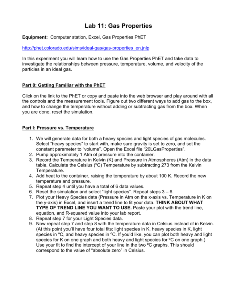
Lab 11: Gas Properties
Equipment: Computer station, Excel, Gas Properties PhET
http://phet.colorado.edu/sims/ideal-gas/gas-properties_en.jnlp
In this experiment you will learn how to use the Gas Properties PhET and take data to
investigate the relationships between pressure, temperature, volume, and velocity of the
particles in an ideal gas.
Part 0: Getting Familiar with the PhET
Click on the link to the PhET or copy and paste into the web browser and play around with all
the controls and the measurement tools. Figure out two different ways to add gas to the box,
and how to change the temperature without adding or subtracting gas from the box. When
you are done, reset the simulation.
Part I: Pressure vs. Temperature
1. We will generate data for both a heavy species and light species of gas molecules.
Select “heavy species” to start with, make sure gravity is set to zero, and set the
constant parameter to “volume”. Open the Excel file “20LGasProperties”.
2. Pump approximately 1 Atm of pressure into the container.
3. Record the Temperature in Kelvin (K) and Pressure in Atmospheres (Atm) in the data
table. Calculate the Celsius (oC) Temperature by subtracting 273 from the Kelvin
Temperature.
4. Add heat to the container, raising the temperature by about 100 K. Record the new
temperature and pressure.
5. Repeat step 4 until you have a total of 6 data values.
6. Reset the simulation and select “light species”. Repeat steps 3 – 6.
7. Plot your Heavy Species data (Pressure in Atm on the x-axis vs. Temperature in K on
the y-axis) in Excel, and insert a trend line to fit your data. THINK ABOUT WHAT
TYPE OF TREND LINE YOU WANT TO USE. Paste your plot with the trend line,
equation, and R-squared value into your lab report.
8. Repeat step 7 for your Light Species data.
9. Now repeat step 7 and step 8 with the temperature data in Celsius instead of in Kelvin.
(At this point you’ll have four total fits: light species in K, heavy species in K, light
species in ºC, and heavy species in ºC. If you’d like, you can plot both heavy and light
species for K on one graph and both heavy and light species for ºC on one graph.)
Use your fit to find the intercept of your line in the two ºC graphs. This should
correspond to the value of “absolute zero” in Celsius.
Part II: Volume vs. Temperature
1. Reset the simulation, and pump some heavy gas into the box. AFTER pumping in
some gas, click the button to hold pressure constant, and open the species information
box.
2. Record how much heavy species you have in your box and the pressure in ATM in the
spreadsheet.
3. First, cool the gas down to about 150K slowly. Use the ruler to measure the width of
the box and record the exact temperature, the width of the box, and the average speed
of the molecules in your spreadsheet.
4. Repeat step 3 five more times after increasing the temperature by about 50K for each
trial.
5. Repeat steps 1-4 for light species.
6. Plot your heavy species data (Width in nm on the x-axis vs. Temperature in K on the yaxis) in Excel, and insert a trend line to fit your data. THINK ABOUT WHAT TYPE OF
TREND LINE YOU WANT TO USE. Paste your plot with the trend line, equation, and
R-squared value into your lab report.
7. Repeat step 6 for your light species data.
8. Now plot your heavy species data (Average velocity on the x-axis vs. temperature on
the y-axis) and insert a trend line. THINK ABOUT WHAT TYPE OF TREND LINE
YOU WANT TO USE. Paste your plot with the trend line, equation, and R-squared
value into your lab report.
9. Repeat step 8 for your light species data.
10. Let’s assume that all the thermal energy in the gas is due solely to the total kinetic
energy of all the gas atoms. Using your data from part II and your prelab, KE = ½ mv2
and Eth = 3/2 NkBT, find the mass in kg of one of the heavy species atoms and one of
the light species atoms (hint: you are looking for m/N in terms of the slope of your
trend line and some other constant numbers).
Analysis/Conclusions
1. What happens when you add too much gas to the box? What happens if you heat the
gas up too much? Explain why this simulation does this in terms of the ideal gas law.
2. What type of trend line did you use to fit your pressure vs. temperature data in Part I?
Explain why you picked this particular trend line.
3. Physically, would it make sense for us to force our trend lines to go through the origin
when using temperature in Kelvin? Explain why or why not.
4. Calculate the percent error in your value for absolute zero in Celsius from both the
heavy species and the light species data (see graphs from Part I step 9). The
accepted value is -273.15º C.
5. What type of trend line did you use to fit your temperature vs. volume data? Explain
why you picked this particular trend line.
6. What type of trend line did you use to fit your temperature vs. average velocity data?
Explain why you picked this particular trend line.
7. What is the intercept of your average velocity vs. temperature plot trend line? Explain
using the concept of absolute zero and the laws of thermodynamics whether your
intercept makes physical sense (hint: is it physically possible to cool a substance down
to absolute zero?).
8. The light species gas is an atomic gas (that is, the individual particles are single atoms
and not two atoms combined into a molecule). Using your answer from step 10 in part
II, which element do you think the light species is?
9. The heavy species gas is a diatomic gas (so the particles are molecules of two atoms
of the same element stuck together). Using your answer from step 10 in part II, which
element do you think the heavy species is?
10. Based on your answers to 8 and 9, do you think the developers of this simulation
primarily consider themselves to be physicists or chemists?