5.3 Test of association
5.4 Measures of association
5.6 Power McNemar’s test
References
5.3 Test of association
5.4 Measures of association
5.6 Power McNemar’s test
References
Outline of the chapter
Biostatistical Methods
SoSe2009
Chapter 5: Case-control and matched studies
Michael Höhle1
1 Department of Statistics
Ludwig-Maximilians-Universität München
1
5.3 Tests of association for matched pairs
2
5.4 Measures of association for matched pairs
3
5.6 Power function of McNemar’s test
8th lecture @ 8 June 2009
Michael Höhle
5.3 Test of association
5.4 Measures of association
BioMeth2009
Michael Höhle
1/ 20
5.6 Power McNemar’s test
References
5.3 Test of association for matched pairs
2/ 20
5.6 Power McNemar’s test
References
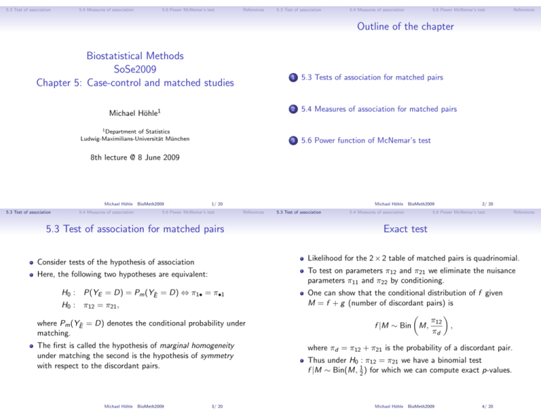
Exact test
To test on parameters π12 and π21 we eliminate the nuisance
parameters π11 and π22 by conditioning.
Here, the following two hypotheses are equivalent:
H0 : P(YE = D) = Pm (YĒ = D) ⇔ π1• = π•1
H0 : π12 = π21 ,
where Pm (YĒ = D) denotes the conditional probability under
matching.
The first is called the hypothesis of marginal homogeneity
under matching the second is the hypothesis of symmetry
with respect to the discordant pairs.
BioMeth2009
BioMeth2009
5.4 Measures of association
Likelihood for the 2 × 2 table of matched pairs is quadrinomial.
Consider tests of the hypothesis of association
Michael Höhle
5.3 Test of association
3/ 20
One can show that the conditional distribution of f given
M = f + g (number of discordant pairs) is
π12
f |M ∼ Bin M,
,
πd
where πd = π12 + π21 is the probability of a discordant pair.
Thus under H0 : π12 = π21 we have a binomial test
f |M ∼ Bin(M, 12 ) for which we can compute exact p-values.
Michael Höhle
BioMeth2009
4/ 20
5.3 Test of association
5.4 Measures of association
5.6 Power McNemar’s test
References
McNemar’s test (1)
5.3 Test of association
5.4 Measures of association
Because the multinomial distribution can be approximated by
a multivariate normal distribution we have
To test the hypothesis H0 : π12 = π21 we look at
d
p = (p11 , p12 , p21 , p22 )0 ≈ N4 (π, Σ),
p12 − p21
ZM = q
d 12 − p21 |H0 )
Var(p
where
p12 − p21
f −g
ZM = p
=√
f +g
(p12 + p21 )/N
Michael Höhle
5.3 Test of association
5.4 Measures of association
BioMeth2009
d
2 ≈
ZM


π11 (1 − π11 )
−π11 π12
−π11 π21
−π11 π22
1  −π11 π12
π12 (1 − π12 )
−π12 π21
−π12 π22 
Σ= 
−π11 π21
−π12 π21
π21 (1 − π21 )
−π21 π22 
N
−π11 π22
−π12 π22
−π21 π22
π22 (1 − π22 )
One can show that
We have asymptotically ZM ≈ N(0, 1) or
References
Aside: Asymptotic normal distribution of π̂
Let (e, f , g , h)0 ∼ M4 (N, π), where π = (π11 , π12 , π21 , π22 )0 .
d
5.6 Power McNemar’s test
χ2 (1).
Note that this distribution is degenerate, because
4
X
pi = 1.
i=1
Michael Höhle
5/ 20
5.6 Power McNemar’s test
References
Example: oral contraceptives and blood clotting (1)
5.3 Test of association
5.4 Measures of association
BioMeth2009
6/ 20
5.6 Power McNemar’s test
References
Example: oral contraceptives and blood clotting (2)
The data:
Example in Sartwell et al. (1969): Suspicion that oral
contraceptives might predispose women towards
thromboembolism.
175 cases from American hospitals during 3-year period with
individually matched controls
Matching criterion: female, discharged alive from the same
hospital in the same 6-month time interval as the case, same
age (5 year span), marital status, race, etc.
Cases and controls were then asked about their use of oral
contraceptives.
Michael Höhle
BioMeth2009
7/ 20
> (sartwell <- matrix(c(10, 13, 57, 95), 2, 2, dimnames = list(c("D-E",
+
"D-notE"), c("notD-E", "notD-notE"))))
D-E
D-notE
notD-E notD-notE
10
57
13
95
Exact test in R:
> binom.test(x = sartwell[1, 2], n = sartwell[1, 2] + sartwell[2,
+
1], p = 0.5, alternative = "two.sided")
Exact binomial test
data: sartwell[1, 2] and sartwell[1, 2] + sartwell[2, 1]
number of successes = 57, number of trials = 70, p-value = 1.029e-07
alternative hypothesis: true probability of success is not equal to 0.5
95 percent confidence interval:
0.7033852 0.8972389
sample estimates:
probability of success
0.8142857
Michael Höhle
BioMeth2009
8/ 20
5.3 Test of association
5.4 Measures of association
5.6 Power McNemar’s test
References
5.3 Test of association
Example: oral contraceptives and blood clotting (3)
5.4 Measures of association
5.6 Power McNemar’s test
References
Conditional Odds ratio (1)
Under matching the marginal odds ratio of matching is not
equivalent to the population odds ratio
McNemar’s test in R:
ORm =
> mcnemar.test(sartwell, correct = FALSE)
McNemar's Chi-squared test
P(YE = D)/P(YE = D)
π1• /π2•
=
6= OR .
π•1 /π•2
Pm (YE = D)/Pm (YE = D)
Instead we look at the conditional OR conditioned on a
specific value z of the matching covariate Z :
data: sartwell
McNemar's chi-squared = 27.6571, df = 1, p-value = 1.448e-07
Hence we reject H0 at almost every significance level: Cases
and control appear to differ in the presence of the exposure
factor.
ORz =
P(YE = D|z) P(YE = D|z)
·
.
P(YE = D|z) P(YE = D|z)
Although P(YE = D|z) and P(YE = D|z) may vary with z we
assume a constant ORz for all values of z, i.e.
ORz = ORC
Michael Höhle
5.3 Test of association
BioMeth2009
5.4 Measures of association
9/ 20
5.6 Power McNemar’s test
Conditional Odds ratio (2)
E
E
D
D
D
π11|z
π21|z
π•1|z
π12|z
π22|z
π•2|z
π1•|z
π2•|z
1
10/ 20
5.6 Power McNemar’s test
References
Exact confidence interval
Large sample confidence interval
where π12 and π21 are the population average discordant
probabilities.
BioMeth2009
BioMeth2009
πf
Then ORC = 1−π
and CIs are computed by
f
logit-transformation of the borders of a CI for πf .
π12 p12
f
=
ˆ
= ,
π21 p21
g
Michael Höhle
5.4 Measures of association
Exact confidence limits for ORC can be based on the
conditional binomial distribution from slide 4, i.e.
f |M ∼ Bin(M, πf ), where πf = π12 /πd and πd = π12 + π21 .
In this setting one can show (→ blackboard)
ORC =
5.3 Test of association
Confidence limits for the conditional odds ratio
Basically we construct a 2 × 2 table for each matched pair
D
Michael Höhle
References
∀z.
11/ 20
A large sample (1 − α) · 100% CI for θ =
plog ORC is obtained
by using θ̂ ± z1−α se(θ̂), where se(θ̂) = M/(fg ).
A back-transformation provides a CI for ORC .
Michael Höhle
BioMeth2009
12/ 20
5.3 Test of association
5.4 Measures of association
5.6 Power McNemar’s test
References
5.3 Test of association
Mantel-Haenszel Analysis (1)
5.4 Measures of association
5.6 Power McNemar’s test
References
Mantel-Haenszel Analysis (2)
Consider the sample of matched pairs as N independent
samples consisting of one member in each exposure group
(E , E ) (prospective) or (D, D) (retrospective).
c MH can be computed by using the
Confidence intervals for OR
d
c MH ).
large sample variance Var(log
OR
The i’th table provides an unmatched 2 × 2 table
E
E
D
ai
bi
m1i
D
ci
di
m2i
n1i = 1 n2i = 1
2
where m1i = 0, 1, 2.
We have that (→ blackboard)
2
XC2 (MH) = XM
,
i.e. the Mantel-Haenszel test statistic equals the squared
McNemar’s test statistic.
However, from our Mantel-Haenszel derivations we also get an
estimator for the OR not just a test.
One can show that (→ blackboard)
c MH = f = OR
c C.
OR
g
Michael Höhle
5.3 Test of association
5.4 Measures of association
BioMeth2009
13/ 20
5.6 Power McNemar’s test
Michael Höhle
References
Mantel-Haenszel Analysis (3)
5.3 Test of association
5.4 Measures of association
14/ 20
5.6 Power McNemar’s test
References
Example: Mantel-Haenszel Analysis (1)
A 1:1 matched case-control study was performed to
investigate the association between tonsillectomy and
Hodgkin’s disease.
Additional remarks:
dC (MH) = OR
dC
We have OR
dC (MH) ) based on the expression
Furthermore, a CI for log(OR
in Chapter 4 corresponds to the large-sample confidence
dC ) from slide 12
interval for log(OR
In Chapter 6 we will see that the estimator for ORC also arises
from a conditional logit model for pair-matched data.
Results of the 85 pairs in the study:
D
E E
E 26 15
D
E
7 37
Using mantelhaen.test for the analysis in R:
> hodgkin <- matrix(c(26, 7,
+
"D-notE"), c("notD-E",
> tables <- array(c(1, 0, 1,
+
1), dim = c(2, 2, 4))
> hodgkin.strata <- tables[,
Michael Höhle
BioMeth2009
BioMeth2009
15/ 20
15, 37), 2, 2, dimnames = list(c("D-E",
"notD-notE")))
0, 1, 0, 0, 1, 0, 1, 1, 0, 0, 1, 0,
, rep(1:4, times = t(hodgkin))]
Michael Höhle
BioMeth2009
16/ 20
5.3 Test of association
5.4 Measures of association
5.6 Power McNemar’s test
References
Example: Mantel-Haenszel Analysis (2)
5.3 Test of association
5.4 Measures of association
5.6 Power McNemar’s test
References
5.6 Unconditional power function of McNemar’s test (1)
McNemar’s test investigates H0 : π12 = π21 vs.
H1 : π12 6= π21 .
Assuming the test statistic is T = p12 − p21 which is
π d
d
TH0 ≈ N 0,
,
πd = π12 + π21 ,
N
d
πd − (π12 − π21 )2
TH1 ≈ N π12 − π21 ,
.
N
> mantelhaen.test(hodgkin.strata, correct = FALSE)
Mantel-Haenszel chi-squared test without continuity correction
data: hodgkin.strata
Mantel-Haenszel X-squared = 2.9091, df = 1, p-value = 0.08808
alternative hypothesis: true common odds ratio is not equal to 1
95 percent confidence interval:
0.8737077 5.2555753
sample estimates:
common odds ratio
2.142857
Michael Höhle
5.3 Test of association
5.4 Measures of association
BioMeth2009
Using the formula from Chapter 3 to compute the necessary
sample size of N matched pairs one obtains:

!2 
p
√
2
z
π
+
z
π
−
(π
−
π
)
1−α
12
21
d
d
1−β
.
N=


π12 − π21


17/ 20
5.6 Power McNemar’s test
Michael Höhle
References
Unconditional power function of McNemar’s test (2)
5.3 Test of association
BioMeth2009
5.4 Measures of association
18/ 20
5.6 Power McNemar’s test
Literature I
To calculate a sample size we need to specify π12 and
OR = π12 /π21 , i.e. π12 = OR · π21 .
Assume π21 = 0.125 and we wish to detect an odds ratio of
OR = 2. Hence π12 = 0.25 and πd = 0.375.
For α = 0.05 the necessary sample size for a two-sided test
with power 1 − β = 0.8 is
Sartwell, P., Masi, A., Arthes, F., Greene, G., and Smith, H. (1969).
Thromboembolism and oral contraceptives: an epidemiologic case-control study.
Am J Epidemiol, 90(5):365–380.
> samsize.mcnemar <- function(pi.12, pi.21, alpha = 0.05, beta = 0.1,
+
sided = 1) {
+
pi.d <- (pi.12 + pi.21)
+
N <- (qnorm(1 - alpha/sided) * sqrt(pi.d) + qnorm(1 - beta) *
+
sqrt(pi.d - (pi.12 - pi.21)^2))^2/(pi.12 - pi.21)^2
+
return(ceiling(N))
+ }
> samsize.mcnemar(pi.12 = 0.125, pi.21 = 0.25, sided = 2)
[1] 248
Michael Höhle
BioMeth2009
19/ 20
Michael Höhle
BioMeth2009
20/ 20
References