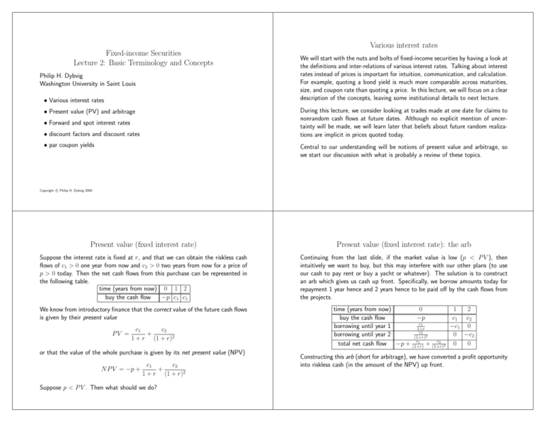
Various interest rates
Fixed-income Securities
Lecture 2: Basic Terminology and Concepts
Philip H. Dybvig
Washington University in Saint Louis
• Various interest rates
• Present value (PV) and arbitrage
• Forward and spot interest rates
• discount factors and discount rates
• par coupon yields
We will start with the nuts and bolts of fixed-income securities by having a look at
the definitions and inter-relations of various interest rates. Talking about interest
rates instead of prices is important for intuition, communication, and calculation.
For example, quoting a bond yield is much more comparable across maturities,
size, and coupon rate than quoting a price. In this lecture, we will focus on a clear
description of the concepts, leaving some institutional details to next lecture.
During this lecture, we consider looking at trades made at one date for claims to
nonrandom cash flows at future dates. Although no explicit mention of uncertainty will be made, we will learn later that beliefs about future random realizations are implicit in prices quoted today.
Central to our understanding will be notions of present value and arbitrage, so
we start our discussion with what is probably a review of these topics.
c Philip H. Dybvig 2000
Copyright Present value (fixed interest rate)
Present value (fixed interest rate): the arb
Suppose the interest rate is fixed at r, and that we can obtain the riskless cash
flows of c1 > 0 one year from now and c2 > 0 two years from now for a price of
p > 0 today. Then the net cash flows from this purchase can be represented in
the following table.
time (years from now) 0 1 2
buy the cash flow
−p c1 c1
Continuing from the last slide, if the market value is low (p < P V ), then
intuitively we want to buy, but this may interfere with our other plans (to use
our cash to pay rent or buy a yacht or whatever). The solution is to construct
an arb which gives us cash up front. Specifically, we borrow amounts today for
repayment 1 year hence and 2 years hence to be paid off by the cash flows from
the projects.
We know from introductory finance that the correct value of the future cash flows
is given by their present value
time (years from now)
0
1
2
buy the cash flow
−p
c 1 c2
c1
borrowing until year 1
−c1 0
1+r
c2
borrowing until year 2
0 −c2
(1+r)2
c1
c2
total net cash flow −p + (1+r) + (1+r)2 0
0
PV =
c2
c1
+
1 + r (1 + r)2
or that the value of the whole purchase is given by its net present value (NPV)
c1
c2
N P V = −p +
+
1 + r (1 + r)2
Suppose p < P V . Then what should we do?
Constructing this arb (short for arbitrage), we have converted a profit opportunity
into riskless cash (in the amount of the NPV) up front.
Deep theoretical insights
• Buy if it’s too cheap.
• Sell if it’s too expensive.
• Use an arb to convert a good deal into pure profit.
Spot rate and forward rates
So far, we have taken the yield curve to be flat; that is, we have assumed that we
can enter commitments now to borrow and lend money a year from now on the
same terms that are available now. That is why the accumulation of interest on
a two-year loan is the same in both years. However, this was just a simplifying
assumption.
In fact, commitments for a year from now will be typically be made at a different
rate than is available now in the spot market. The spot rate is the rate at which
we borrow and lend now for payment a year from now. The rates at which we
commit for borrowing and lending in different future years are forward rates.
We need to fix notation to quantify these things. We will denote by r t the spot
rate quoted at t−1 for lending until t. And, we will denote by f (s, t) the forward
rate quoted at time s for lending from t − 1 to t in the future. It is useful to
think of the spot rate as a trivial case of forward rate, that is, r t = f (t − 1, t).
A plot of an interest rate against maturity is called a yield curve. One yield curve
is the yield curve in forward rates. We will encounter other yield curves later.
PV with a nontrivial yield curve
NPV with a nontrivial yield curve
One general expression for the present value with a nontrivial yield curve has
discounting by each of the one-period forward rates in turn. If we have a riskless
cash flow that will pay c1 one year hence, c2 two years hence, c3 three years
hence, etc., then the present value is
The NPV includes the initial cash flow. If we have that p is the purchase price
so that c0 = −p is the initial cash flow, then the net present value is, as usual,
NP V = P V − p
c1
c2
PV =
+
1 + f (0, 1) (1 + f (0, 1))(1 + f (0, 2))
cT
+ ... +
(1 + f (0, 1))(1 + f (0, 2))...(1 + f (0, T ))
T
ct
X
=
Qt
t=1 s=1 (1 + f (0, s))
where
P
indicates a sum of terms and
Q
indicates a product.
=
T
X
t=0
ct
s=1 (1 + f (0, s))
Qt
where an empty product is defined to equal 1.
PV: the arb
In-class exercise: the PV arb
Suppose cash flows of c1 a year hence and c2 two years hence are selling for the
bundled price of p, and this price is larger than the present value computed using
spot and forward rates f (0, 1) = r1 and f (0, 2) = r2. Then we can sell the cash
flows in the market (because they are too expensive) and convert this profitable
opportunity into cash up front using the following arb.
Suppose the market price is 150 for a security paying 100 a year from now and
90 two years from now. Further suppose that the spot one-year rate is 25% and
the forward rate for lending from one year out to two years out is 20%.
time (years from now)
0
1
2
sell the cash flow
p
−c1
−c2
c1
c2
2
spot lending
− 1+r
− (1+r1c)(1+r
c1 + 1+r
0
1
2)
2
c2
forward lending
0
− 1+r2
c2
c1
c2
total net cash flow p − 1+r
−
0
0
(1+r1 )(1+r2 )
1
• How do we profit from the discrepancy between the market price and PV?
The bad news
At this point, it may seem that we have arrived at a very cheerful state of affairs:
after a few simple calculations we buy and sell and pocket cash. Unfortunately,
things are not so easy.
• Absence of arbitrage is the norm.
• Compute the PV and NPV of the cash flow.
• Construct an arb to convert the profit into a sure thing.
time (years from now) 0
1
2
sell the cash flow
150 −100 −90
Present value using zero-coupon bonds
• add up prices times quantities as at the grocery
• discount factor D(s, t): price at date s of getting $1 at some subsequent
date t
• Most arbs still involve some risk-taking.
• Look at the corresponding zero-coupon (or bullet or pure-discount) bond with
face F and price P
• Many smart people are looking for arbs; finding simple arbs is especially rare.
• D(s,t) = P/F
For finance scholars, our theory usually assumes there is no arbitrage, and p =
P V . When our theory is wrong, we do not feel so bad, because then we can
make money by trading.
Denote by ct the cash flow at t. Then, the present value and net present value
are given by the following formulas.
PV =
T
X
t=1
NP V =
D(0, t)ct
T
X
t=0
D(0, t)ct
Present value using zero-coupon bonds: the arb
Zero-coupon prices and yields
Consider the following scenario. A marketed claim is a riskless self-amortizing
loan that pays $100 a year from now and $100 two years from now and is priced
at $165 in the market. A zero-coupon bond maturing one year from now costs 90
cents per dollar of face value, while a zero-coupon bond maturing two years from
now costs 80 cents per dollar of face value. This means that the self-amortizing
loan has a present value of .9 × $100 + .8 × $100 = $170. Since the market price
is less than the PV, this claim is cheap and we should buy it. Here are the cash
flows:
For any bond, its yield is the fixed interest rate that would make the bond price
equal to the present value of its cash flows. Therefore, the yield z(s,t) at time s
on a zero (a zero-coupon bond) maturing at a later date t solves the equation
time (years from now)
0
1
2
buy the cash flow
−165 100 100
borrowing until year 1 90 −100 0
borrowing until year 2 80
0 −100
total net cash flow
5
0
0
Again, the arb converts a good deal into pure profit.
Institutional note The approximation is similar to, but different from, the
formula


dtm 

P = F 1 − d
360
used in practice to relate a Treasury Bill discount d to its price P , face value F
and days-to-maturity dtm. This formula is not an approximation, and instead
it defines what price corresponds to the quoted yield. Note that 360 is not an
approximation to the number of days in the year; Treasury discounts are defined
in terms of an artificial 360-day year.
D(s, t) =
1
(1 + z(s, t))t−s
where D(s, t) is the corresponding discount factor, so that
z(s, t) = D(s, t)−1/(t−s) − 1
1 − D(s, t)
≈
t−s
The approximation is best for short maturities (small t − s) and small rates.
In-class exercise: discount factors
Given the spot one-year interest rate of 20% and a one-year forward interest rate
of 25%, what are the one-year and two-year discount factors? What are the
one-year and two-year zero-coupon yields?
Implied forward rates
Implied forward rates: the arb
In the market, we see active quotes of discount bonds (Treasury STRIPs) rather
than the forward borrowing and lending rates. However, we can replicate forward
borrowing to obtain an implied forward rate from the STRIP curve. For example,
if we want to borrow $2 million for one year, two years out, we buy $2 million
face of STRIPs maturing in two years, and we sell short an equivalent dollar
value (today) of STRIPs maturing in three years. Given D(0, 2) and D(0, 3), we
would buy $2 million face of 2-year strips worth $2D(0, 2) today, which would
be paid for using $2D(0, 2)/D(0, 3) face of 3-year strips. The implied forward
rate would therefore be (2D(0, 2)/D(0, 3) − 2)/2 = D(0, 2)/D(0, 3) − 1. The
general formula is
Of course, whenever there is a replicating portfolio there is an implicit arb if prices
are out of line. For example, suppose we can borrow and lend forward one year
from now at 10%, and that the discount factor is 90% one year out and 80%
two years out. Then the implied forward rate is .9/.8 − 1 = .125, which means
(borrowing) money is too cheap, so we should buy. At the scale of $1, the arb is:
f (s, t) =
time (years from now) 0
1
2
borrow forward
0
1 −1.1
sell one-year zero
.9 −1 0
buy two-year zero
−.88 0 1.1
total net cash flow
0.02 0
0
D(s, t − 1)
−1
D(s, t)
Coupon bond yields
In-class exercise: par coupon yields
The yield on a coupon bond is the interest rate that makes its price equal to its
present value. If a bond has price P , T remaining coupons of c per period, and
face value F (paid at the maturity T periods from now), then the yield y solves
the equation
A coupon bond maturing in two years has a face value of $112 million and an
annual coupon of $8 million per year. If its yield is 20%, what is its price now?
(The coupon this year has already been paid, so the price does not include a
claim to the coupon now.)
P =
T
F
c
X
+
T
s=1 (1 + y)s
(1 + y)
We often talk of the moneyness of a bond. A bond sells at a discount if its price
is less than its face value, at par if its price is equal to its face value, or at a
premium if its price is greater than its face value.
Institutional note In practice, most coupon bonds pay coupons twice a year.
For this reason, bond yields are customarily computed using half-year rates with
interpolation for fractions of half-years. The rates are quoted as annual rates,
defined to be twice the half-year rates. Also, bonds are traded with accrued
interest so the price does not jump at coupon dates.
Par coupon bond yields
Often when we hear about the yield curve, the speaker has in mind a plot of
coupon bond yields against maturity. However, there is no reason in general
why different coupon bonds with the same maturity would have exactly the same
yield; in fact this would be the exception rather than the rule. Therefore, when
people talk about the yield curve for coupon bonds, they have not really pinned
it down. Talking about the par coupon bond yield pins it down.
To compute a par coupon yield from discount factors, we first note that the yield
y is the same as the coupon yield c/F for a par coupon bond, that is,
F =
T
F
c
X
+
(1 + y)T s=1 (1 + y)s
implies y = c/F (as can be proven using the annuity formula). Now,
F = F D(0, T ) +
T
X
s=1
yF D(0, s),
so that
y=
1 − D(0, T )
PT
s=1 D(0, s)