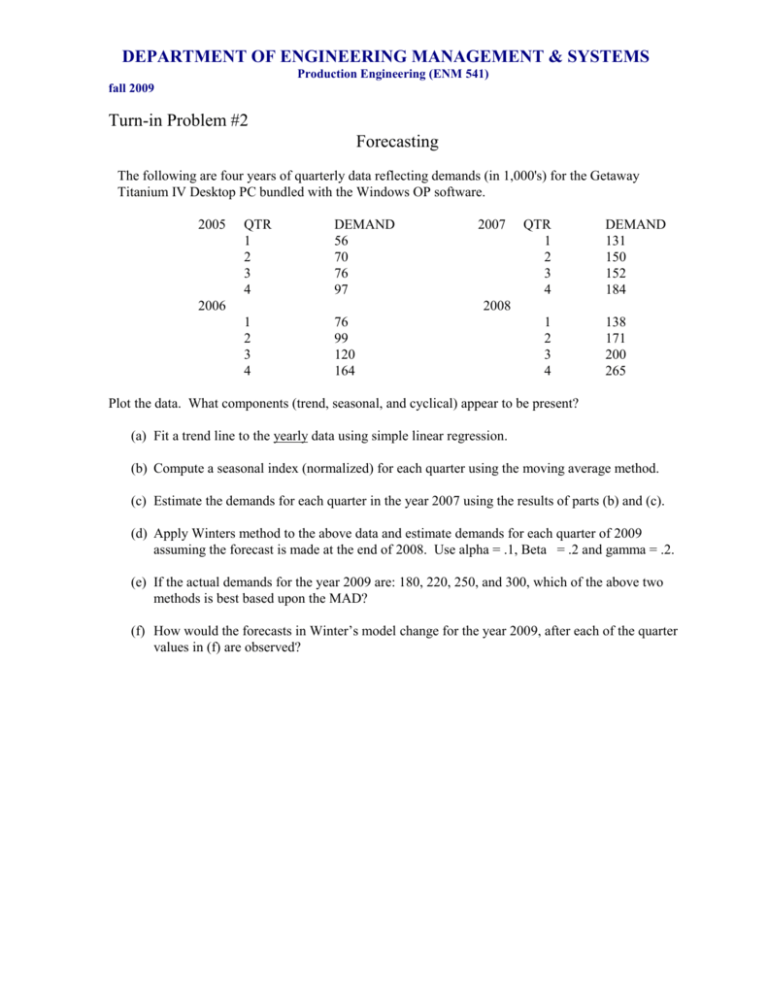
DEPARTMENT OF ENGINEERING MANAGEMENT & SYSTEMS
Production Engineering (ENM 541)
fall 2009
Turn-in Problem #2
Forecasting
The following are four years of quarterly data reflecting demands (in 1,000's) for the Getaway
Titanium IV Desktop PC bundled with the Windows OP software.
2005
QTR
1
2
3
4
DEMAND
56
70
76
97
2006
2007
QTR
1
2
3
4
DEMAND
131
150
152
184
2008
1
2
3
4
76
99
120
164
1
2
3
4
138
171
200
265
Plot the data. What components (trend, seasonal, and cyclical) appear to be present?
(a) Fit a trend line to the yearly data using simple linear regression.
(b) Compute a seasonal index (normalized) for each quarter using the moving average method.
(c) Estimate the demands for each quarter in the year 2007 using the results of parts (b) and (c).
(d) Apply Winters method to the above data and estimate demands for each quarter of 2009
assuming the forecast is made at the end of 2008. Use alpha = .1, Beta = .2 and gamma = .2.
(e) If the actual demands for the year 2009 are: 180, 220, 250, and 300, which of the above two
methods is best based upon the MAD?
(f) How would the forecasts in Winter’s model change for the year 2009, after each of the quarter
values in (f) are observed?
DEPARTMENT OF ENGINEERING MANAGEMENT & SYSTEMS
Production Engineering (ENM 541)
fall 2009
Turn-in Problem #2
Forecasting
Note: Solutions will be submitted via a web submission page found on the course website.
(a) list
components
(b) trendline
Intercept:
Slope:
Yr 2007 estimate:
Qtr1
Qtr2
Qtr3
Qtr4
Qtr1
Qtr2
Qtr3
Qtr4
Qtr3
Qtr4
Qtr3
Qtr4
(c) Indices
(d) yr 2009 demands
(e) Winter’s model
S0
(e) Winter’s model initial indices
Qtr1
Qtr2
Qtr3
Qtr4
(e) Winters model
yr 2009 demands
G0
Qtr1
Qtr2
Model (b)-(d)
Winters Model
(f) MAD
(g) Revised Winter’s forecasts
Qtr2