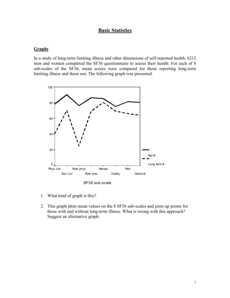
Basic Statistics
Graphs
In a study of long-term limiting illness and other dimensions of self-reported health, 6212
men and women completed the SF36 questionnaire to assess their health. For each of 8
sub-scales of the SF36, mean scores were compared for those reporting long-term
limiting illness and those not. The following graph was presented.
100
SF36 score
80
60
40
20
Not ill
0
Phys fun
Long term ill
Role phys
Soc f un
Role emo
Mental
Pain
Vitality
General
SF36 sub-scale
1. What kind of graph is this?
2. This graph plots mean values on the 8 SF36 sub-scales and joins up points for
those with and without long-term illness. What is wrong with this approach?
Suggest an alternative graph.
1
Summarizing Data I
In a study to compare immediate vs. delayed radiotherapy in patients with lung cancer,
data were obtained on activity level scores using the Rotterdam symptom checklist.
Month
0
1
2
4
6
% with symptom score > 10
Immediate treatment
Delayed treatment
45% (49/109)
43% (47/110)
47% (28/59)
48% (39/81)
43% (22/51)
51% (26/51)
49% (24/49)
57% (33/58)
48% (17/35)
64% (31/49)
What is the interpretation of the results shown in the above table?
Summarizing Data II:
The table below shows data from a study of semen analysis and donor success in a
programme of artificial insemination by donor (AID). From the data presented, do you
think it likely that semen count and % motility have Normal distributions?
Semen indices in most and least fertile donors
Successful donors
Unsuccessful donors
No.
Mean (SD)
No.
Mean (SD)
6
Semen count (10 /ml)
18
146.4 (95.7)
19
124.8 (81.8)
% motility
17
60.7 (9.7)
19
58.5 (12.8)
2
Confidence Intervals:
In a study of bone density and falls in older women, 118 volunteers were randomized to
receive either calcium supplements plus a program of exercise classes or to calcium alone
for 2 years. Twelve subjects dropped out from the calcium group and 14 from the calcium
group taking exercise, leaving 92 subjects who completed the two-year project. The
percentage change in bone mineral content and bone mineral density in two years was
calculated for each individual. The authors reported that for the ultradistal forearm the
change in bone mineral content was –2.6 (95% CI –4.6 to –0.6) in the calcium only group
and 1.14 (95% CI –0.8 to 3.1) in the calcium group taking exercise.
1. What do the confidence intervals for the change in bone mineral content mean?
2. To what population do they refer?
3. Confidence intervals are presented for each group separately. Suggest a more
informative confidence interval.
Significance Tests:
Shortly after the grounding of the Braer oil tanker off the Shetland Isles, a study was
conducted to ascertain whether the respiratory tracts of children were being affected by
the crude oil vapour and droplet spray. Peak expiratory flow rate (PEFR) of 44 children
aged 5-12 years was measured twice: 3 days after the shipwreck and 9-12 days after
when the strong smell of oil had abated. Statistical analysis of the paired PEFRs (by
Student’s paired t-test) showed no significant difference between the two sets of values
(P=0.502).
1. What is meant by no significant difference?
2. What is meant by a paired t-test? What assumptions are involved and are they
likely to be justified here?
3. What can we conclude about the effect of spillage on the respiratory function of
children?
3
Correlation
In a randomized placebo-controlled trial of human recombinant growth hormone (rhGH)
in patients with chronic heart failure, 50 patients were allocated to treatment or placebo.
The figure below shows the relationship between changes in serum IGF-1 ( a growth
factor) and changes in left-ventricular mass by treatment group. The authors reported
that, “..a significant relation was found between changes in serum IGF-1 concentrations
and left-ventricular mass for all patients (r = 0.55, p=0.0001) but this relation was less
evident when the two groups were analysed separately (rhGH: r=0.28, p=0.19; placebo:
r=0.36, p=0.08)”
120
100
80
60
40
20
0
-20
placebo
-40
-200
rhGH
-100
0
100
200
Change in IGF-1 (ng/ml)
Suggest why the relation between changes in IGF-1 and changes in left-ventricular
mass as shown in the graph was, “..less evident when the two groups were analysed
separately”.
4
Solutions:
Graphs
1. This is a line graph. Such graphs are usually used to show change in a quantity
over time, which is not the case here.
2. The 8 SF36 sub-scales are discrete scales, not a continuous scale and so to join
them up is meaningless. It suggests some ordering which is not present. A better
graph is one where the subscales are displayed separately, like the bar graph
below. This allows us to compare mean values for those with and without longterm illness on each sub-scale separately.
100
SF36 score
80
60
40
20
Not ill
0
Long term ill
Phys fun
Role phys
Soc f un
Mental
Role emo
Pain
Vitality
General
SF36 sub-scale
5
Summarizing Data I
Looking at the simple percentages alone, it appears that the symptom scores for the
delayed treatment group are increasing over time, whereas those for the immediate
treatment group are static. However, it is clear that the attrition rate in the study is very
high. At six months, data on activity level are presented for less than half of the original
sample. The attrition rate is much higher in the immediate treatment group. The reasons
for dropping out of the study may be different for the two groups. Hence, a simple
comparison of the percentages cannot be made, and more information on the drop-outs
needs to be obtained before the results can be interpreted.
Summarizing Data II
For data that follow a Normal distribution, 2.5% of the observations will lie below the
mean minus 2 standard deviations. Here this would imply negative values for semen
count, which are impossible. Hence we conclude that it is unlikely that semen count
follows a Normal distribution. With % motility, the standard deviation is much less than
half the mean and so the mean minus 2 standard deviations is a possible value. Hence the
data could follow a Normal distribution but without seeing all the observations we cannot
be sure.
Confidence Intervals
1. The two confidence intervals give us a range of values within which the mean
change is estimated to lie in the whole population of women who would volunteer
if they were to receive the treatment for that group. The confidence interval for
the calcium only group tells us that the mean percentage change is a reduction in
bone mineral content somewhere between 0.6 and 4.6 percentage points. For the
calcium plus exercise group the mean percentage change could be a reduction of
0.8 percentage points or an increase of 3.1 percentage points or any value between
these limits.
2. These women were volunteers and it is therefore difficult to extrapolate the
findings to a general population.
3. The confidence intervals provide estimates of the mean change in bone density
over 2 years. Since we are here interested in any effect of exercise on this, a
confidence interval for the difference between the two groups would be more
useful than the two separate intervals provided. Using the data given the
difference in mean change is 3.7 with an approximate 95% CI 0.9 to 6.5. This CI
does not contain the value zero, hence we can infer that the calcium only group
had a significantly higher reduction in bone mineral content compared to the
calcium plus exercise group.
6
Significance tests
1. No significant difference is the result of a significance test comparing PEFR in
children at two points in time after exposure. The null hypothesis is that there is
no change in PEFR in the population from which the sample of children was
drawn. The data were used to give a test statistic that has a known distribution if
the null hypothesis is true. We then find the probability of data as or more
extreme as that observed if the null hypothesis were true. If the probability is
small, then we have good evidence against the null hypothesis. Conventionally,
we use p=0.05 as the cut-off. Here the probability is > 0.05, therefore we
conclude that the study failed to detect a difference. This does not necessarily
mean that no difference exists since we cannot prove that the null hypothesis is
true on the basis of a significance test.
2. The paired t-test is used to test the null hypothesis of no change. It is used here
because we have two measurements on each subject at two points in time and we
are interested in the differences between individuals. It requires the assumption
that the differences follow a Normal distribution. This is likely to be true because
PEFR follows a Normal distribution and the difference of two variables from
Normal distributions will also follow a Normal distribution.
3. There is no evidence for a reduction in lung function in the children between 3
and 12 days after the spillage. However, we should not conclude that the spillage
had no effect on lung function. There may be an effect that is too small to be
statistically significant in a sample of this size. Alternatively, lung function may
have already been reduced before the initial reading was taken and remained
reduced.
Correlation
In this study we have two separate groups, rhGH and placebo, in which the
distributions of IGF-1 hardly overlap. It appears that the rhGH treatment has
increased both IGF-1 and left-ventricular mass. Putting the two groups together in
this way increases the range of the data and so increases the size of the correlation. It
also produces a mixture of two populations, treated and untreated. The relationship
between IGF and mass at the individual level is confused with that at the group level,
an effect similar to that produced by combining multiple observations from each
subject. It is, therefore, misleading to calculate a correlation coefficient for the
combined data.
7