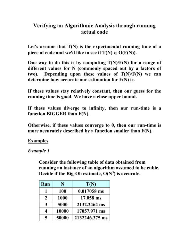
Verifying an Algorithmic Analysis through running
actual code
Let's assume that T(N) is the experimental running time of a
piece of code and we'd like to see if T(N)  O(F(N)).
One way to do this is by computing T(N)/F(N) for a range of
different values for N (commonly spaced out by a factors of
two). Depending upon these values of T(N)/F(N) we can
determine how accurate our estimation for F(N) is.
If these values stay relatively constant, then our guess for the
running time is good. We have a close upper bound.
If these values diverge to infinity, then our run-time is a
function BIGGER than F(N).
Otherwise, if these values converge to 0, then our run-time is
more accurately described by a function smaller than F(N).
Examples
Example 1
Consider the following table of data obtained from
running an instance of an algorithm assumed to be cubic.
Decide if the Big-Oh estimate, O(N3) is accurate.
Run
1
2
3
4
5
N
100
1000
5000
10000
50000
T(N)
0.017058 ms
17.058 ms
2132.2464 ms
17057.971 ms
2132246.375 ms
T(N)/F(N) = 0.017058/(100*100*100) = 1.0758  10-8
T(N)/F(N) = 17.058/(1000*1000*1000) = 1.0758  10-8
T(N)/F(N) = 2132.2464/(5000*5000*5000) = 1.0757  10-8
T(N)/F(N) = 17057.971/(10000*10000*10000) = 1.0757 
10-8
T(N)/F(N) = 2132246.375/(50000*50000*50000) = 1.0757 
10-8
The calculated values converge to a positive constant
(1.0757  10-8) – so the estimate of O(n3) is a good
estimate.
Example 2
Consider the following table of data obtained from
running an instance of an algorithm assumed to be
quadratic. Decide if the Big-Oh estimate, O(N2) is
accurate.
Run
1
2
3
4
5
N
T(N)
100
0.00012 ms
1000
0.03389 ms
10000
10.6478 ms
100000 2970.0177 ms
1000000 938521.971 ms
T(N)/F(N) = 0.00012/(100 * 100) = 1.6  10-8
T(N)/F(N) = 0.03389/(1000 * 1000) = 3.389  10-8
T(N)/F(N) = 10.6478/(10000 * 10000) = 1.064  10-7
T(N)/F(N) = 2970.0177/(100000 * 100000) = 2.970  10-7
T(N)/F(N) = 938521.971/(1000000 * 1000000) =9.385 10-7
The values diverge, so O(n2) is an underestimate.
Limitations of Big-Oh Notation
1) not useful for small sizes of input sets
2) omission of the constants can be misleading – example
2NlogN and 1000N, even though its growth rate is larger the
first function is probably better. Constants also reflect things
like memory access and disk access.
3) assumes an infinite amount of memory – not trivial when
using large data sets
4) accurate analysis relies on clever observations to optimize
the algorithm.
Growth Rates of Various Functions
The table below illustrates how various functions grow with
the size of the input n.
Assume that the functions shown in this table are to be
executed on a machine which will execute a million instructions
per second. A linear function which consists of one million
instructions will require one second to execute. This same
linear function will require only 410-5 seconds (40
microseconds) if the number of instructions (a function of
input size) is 40. Now consider an exponential function.
log
n
0
n
n
n log n
n2
n3
2n
1
1
0
1
1
2
1
1.4
2
2
4
8
4
2
2
4
8
16
64
16
3
2.8
8
24
64
512
256
4
4
16
64
256
4096
65,536
5
5.
3
6
5.7
32
160
1024
32,768
4.294109
40
212
1600
64000
1.0991012
8
64
384
4096
262,144
1.8441019
~10
31.6
1000
9966
106
109
NaN =)
6.3
The Growth Rate of Functions (in terms of steps in the
algorithm)
When the input size is 32 approximately 4.3109 steps will be
required (since 232 = 4.29109). Given our system performance
this algorithm will require a running time of approximately
71.58 minutes. Now consider the effect of increasing the input
size to 40, which will require approximately 1.1x1012 steps
(since 240 = 1.09x1012). Given our conditions this function will
require about 18325 minutes (12.7 days) to compute. If n is
increased to 50 the time required will increase to about 35.7
years. If n increases to 60 the time increases to 36558 years
and if n increases to 100 a total of 4x1016 years will be needed!
Suppose that an algorithm takes T(N) time to run for a
problem of size N – the question becomes – how long will it
take to solve a larger problem? As an example, assume that
the algorithm is an O(N3 ) algorithm. This implies:
T(N) = cN3.
If we increase the size of the problem by a factor of 10 we have:
T(10N) = c(10N)3. This gives us:
T(10N) = 1000cN3 = 1000T(N) (since T(N) = cN3)
Therefore, the running time of a cubic algorithm will increase
by a factor of 1000 if the size of the problem is increased by a
factor of 10. Similarly, increasing the problem size by another
factor of 10 (increasing N to 100) will result in another 1000
fold increase in the running time of the algorithm (from 1000
to 1106).
T(100N) = c(100N)3 = 1106cN3 = 1106T(N)
A similar argument will hold for quadratic and linear
algorithms, but a slightly different approach is required for
logarithmic algorithms. These are shown below.
For a quadratic algorithm, we have T(N) = cN2. This implies:
T(10N) = c(10N)2. Expanding produces the form: T(10N) =
100cN2 = 100T(N). Therefore, when the input size increases by
a factor of 10 the running time of the quadratic algorithm will
increase by a factor of 100.
For a linear algorithm, we have T(N) = cN. This implies:
T(10N) = c(10N). Expanding produces the form: T(10N) =
10cN = 10T(N). Therefore, when the input size increases by a
factor of 10 the running time of the linear algorithm will
increase by the same factor of 10.
In general, an f-fold increase in input size will yield an f 3-fold
increase in the running time of a cubic algorithm, an f 2-fold
increase in the running time of a quadratic algorithm, and an
f-fold increase in the running time of a linear algorithm.
The analysis for the linear, quadratic, cubic (and in general
polynomial) algorithms does not work when in the presence of
logarithmic terms.
When an O(N logN) algorithm experiences a 10-fold increase
in input size, the running time increases by a factor which is
only slightly larger than 10. For example, increasing the input
by a factor of 10 for an O(N logN) algorithm produces: T(10N)
= c(10N) log(10N). Expanding this yields: T(10N) = 10cN
log(10N) = 10cN log10 + 10cN logN = 10T(N) + cN (where c =
10clog10). As N gets very large, the ratio T(10N)/T(N) gets
closer to 10 (since cN/T(N)  (10 log10)/logN gets smaller and
smaller as N increases.
The above analysis implies, for a logarithmic algorithm, if the
algorithm is competitive with a linear algorithm for a
sufficiently large value of N, it will remain so for slightly larger
N.