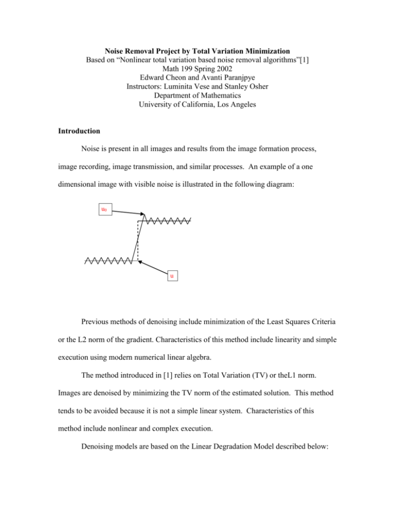
Noise Removal Project by Total Variation Minimization
Based on “Nonlinear total variation based noise removal algorithms”[1]
Math 199 Spring 2002
Edward Cheon and Avanti Paranjpye
Instructors: Luminita Vese and Stanley Osher
Department of Mathematics
University of California, Los Angeles
Introduction
Noise is present in all images and results from the image formation process,
image recording, image transmission, and similar processes. An example of a one
dimensional image with visible noise is illustrated in the following diagram:
u0
u
Previous methods of denoising include minimization of the Least Squares Criteria
or the L2 norm of the gradient. Characteristics of this method include linearity and simple
execution using modern numerical linear algebra.
The method introduced in [1] relies on Total Variation (TV) or theL1 norm.
Images are denoised by minimizing the TV norm of the estimated solution. This method
tends to be avoided because it is not a simple linear system. Characteristics of this
method include nonlinear and complex execution.
Denoising models are based on the Linear Degradation Model described below:
uo(x,y) = u(x,y) + n(x,y), where:
uo(x,y) = noisy image
u(x,y) = clear image
n(x,y) = additive noise
Minimization Problem
Minimization problems for noise removal assume that the mean of the noise is 0.
i.e.:  n(x,y)dxdy = 0 where  = [0,a]x[0,b]
Since the mean of the noise n(x,y) is 0, and integrating both sides over  in the Linear
Degradation Model uo = u + n, or uo – u = n we obtain
 uo =  u.
Using the standard deviation of noise, which shows the intensity of the noise let:
 n2 = 2
Therefore,
 (uo – u)2 =  n2 = 2 (1)
Now take the local averaging around the image except at the boundary, which causes
blurring. In general, the definition of averaging leads to:
u(t,x,y) = u(0,x,y) = uo (x,y) at t=0
du/dt = u = uxx + uyy
Note: uxx + uyy is the Laplace equation, which has a strong smoothing effect.
e.g.: for t=0:
for t=Δt:
for t=2 Δt:
Previous methods have tried to minimize:
Min F(u) = ½  (ux2 + uy2)dxdy
Taking the derivative, we obtain the Laplace equation, which smoothes the image beyond
recognition:
du/dt = u = uxx + uyy
ie: diagram with t=2t. From this, we see that if there is a large jump (gradient), it
includes the jump in the average, causing the smoothing.
To overcome this smoothing problem, we introduce a limit of averages:
Let M be a bound. Looking at the image, we want to take the local average only where
the |derivative of uo(x)|  M
Using our example:
|uo’(x1)|  M
|uo’(x2)| >> M
|uo’(x3)|  M
x1
x2
x3
In essence, we’ve changed the problem of minimizing F(u) to:
F(u) =  (ux2 + uy2)1/2 dxdy (2).
This new method combines the previous linear method constraint (1) with the nonlinear
constraint (2) giving us:
Min F(u) =   (uo – u)2 dxdy +(ux2 + uy2)1/2 dxdy
Note that  is the Lagrange Multiplier, the parameter coefficient which weighs how much
smoothing we have.
Now since we are minimizing F(u), we take the derivative of F, which gives:
F’(u) = 0 =>  (u-uo) = d/dx ( ux/ (ux2 + uy2)1/2 ) + d/dy ( uy/ (ux2 + uy2)1/2 ) (3)
Letting the gradient = |u| = (ux2 + uy2)1/2:
If the gradient is 1, then we obtain the Laplace equation:
(d/dx (ux) + d/dy (uy))
If the gradient is large >>1, then each term goes to 0.
The Numerical Scheme
This formula has the same form as (3) b/c it utilizes an iterative method/scheme,
which can be step up with the following criteria:
Where each position on the graph is represented by an element of a m x n matrix
(ui,j) = [u11…..u1n
un1…..unn]
Each (i,j) = pixel = discrete points.
uij = intensity of light at each point (i,j) on a gray scale where 0(black)<uij<255 (white).
From this we know that the image = function.
(x,y)  u(x,y) on the domain .
Now let h = space step = x = y.
Let (xo,yo) = (0,0).
xi = i*h, yj = j*h (discrete form)
u(xi, yj) = u(i*h, j*h) = uijh
Therefore, obtaining (3).
Results
We used the two dimensional denoising algorithm of [1] on the following images.
To provide a contrast and to grasp a better understanding of the difference between
previous mevthods involving the least squares criteria and the method involved total
variation, we have provided the results of applying previous methods.
image [a] is the original noisy image
Between the methods of Total Variation and Least Squares criteria, we decided to
work with the Total Variation method and minimize the function:
Min F(u) =   (uo – u) 2 dxdy +  (ux2 + uy2) 1/2 dxdy
In order to denoise the noisy image, we used the theory above in order to write an
algorithm that could be utilized practically. In the algorithm, to produce the total
variation image, we used the method described above and introduced in [1].
image [b] created with parameters: lambda = 0.01, iterations = 500
To compare the total variation method with other methods, we manipulated the
least squares criteria and minimize the function:
Min F(u) =   |uo – u| dxdy + (ux2 + uy2) 1/2 dxdy.
Because the absolute value function |.| is not differentiable in 0, we regularize the above
functional using a small parameter  = 0.000001, as follows:
Min F(u) =   [(uo – u)2 + 2] 1/2 dxdy + (ux2 + uy2 + 2 )1/2 dxdy.
Here we can see that although most of the noise has been taken out, the corners of the
objects in the image are slightly rounded and some blurring does occur.
image [c] created with parameters: lambda = 0.1, iterations = 500
To produce another image of comparison we once again manipulate the least
squares criteria and minimized the function:
Min F(u) = [  (uo – u)2 dxdy] 1/2 +  (ux2 + uy2) 1/2 dxdy.
Because the involved functions are not differentiable in zero, again we introduce a small
parameter (to avoid division by zero after differentiation), as follows:
Min F(u) = [ 2 +  (uo – u)2 dxdy] 1/2 +  (ux2 + uy2+ 2 )1/2 dxdy.
After experimenting the parameters lambda and the number of iterations, although the
image somewhat less noisy, it is still not clear (image [d]). We have tried increasing and
decreasing the value of lambda as well as the number of iterations.
image [d] created with parameters: lambda = 112, iterations = 500
Works Cited
[1]
L.I. Rudin, S. Osher and E. Fatemi, “Nonlinear total variation based noise
removal algorithms”, Physica D 60 pp. 259-268 (1992)