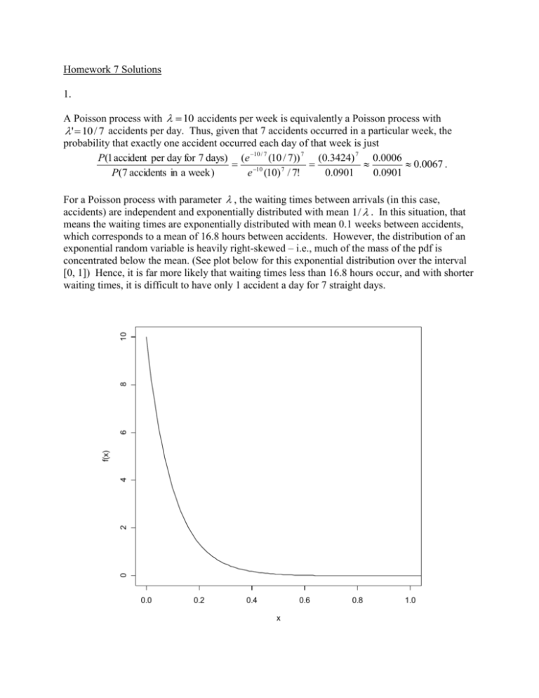
Homework 7 Solutions
1.
A Poisson process with   10 accidents per week is equivalently a Poisson process with
 ' 10 / 7 accidents per day. Thus, given that 7 accidents occurred in a particular week, the
probability that exactly one accident occurred each day of that week is just
P(1 accident per day for 7 days) (e 10 / 7 (10 / 7)) 7 (0.3424) 7 0.0006
 10


 0.0067 .
P(7 accidents in a week )
0.0901
0.0901
e (10) 7 / 7!
0
2
4
f(x)
6
8
10
For a Poisson process with parameter  , the waiting times between arrivals (in this case,
accidents) are independent and exponentially distributed with mean 1/  . In this situation, that
means the waiting times are exponentially distributed with mean 0.1 weeks between accidents,
which corresponds to a mean of 16.8 hours between accidents. However, the distribution of an
exponential random variable is heavily right-skewed – i.e., much of the mass of the pdf is
concentrated below the mean. (See plot below for this exponential distribution over the interval
[0, 1]) Hence, it is far more likely that waiting times less than 16.8 hours occur, and with shorter
waiting times, it is difficult to have only 1 accident a day for 7 straight days.
0.0
0.2
0.4
0.6
x
0.8
1.0
2. Ross 5.37 p. 251
a) If X is uniformly distributed over (-1, 1), then we have
 0.5,  1  x  1
f ( x)  
otherwise
0,
Hence, the probability that X  0.5 is
P( X  0.5)  P( X  0.5)  P( X  0.5)  0.25  0.25  0.5 .
b) To find the density function of X :
F X (a)  P( X  a)  P(a  X  a)  a , where 0  a  1 .
Taking the derivative of this with respect to a gives us
dF X (a)
f X (a) 
 1 , where 0  a  1 .
da
In other words, X is uniformly distributed on (0, 1).
3. Ross 5.41 p. 251
We have that  is uniformly distributed on ( / 2,  / 2) . If R  A sin(  ) , then to find the
distribution of R, we just find the cdf for R as a function of x and then take the derivative with
respect to x to obtain the pdf.
x

FR ( x)  P( R  x)  P( A sin(  )  x)  P sin(  )  
A


d 1
 x 
x 1
 P  arcsin    
 arcsin   

 
 A 
 A 2

 / 2
dF ( x)
1
 f R ( x)  R

, where x  A
dx
 A2  x 2
arcsin(x / A )
4. Ross 6.6 p. 313
5
There are a total of    10 different sequences in which the 5 transistors (2 defective) can be
 2
drawn from the bin. Each of these sequences is equally likely to occur, so the joint pdf of N1
and N 2 is just
1
P( N1  i, N 2  j )  , i  1, , 4; j  1, , 5  i
10
5. Ross 6.11 p. 314
The customers can be viewed as draws from a multinomial distribution where p1  0.45 is the
probability of an “ordinary” purchaser, p2  0.15 is the probability of a “plasma” purchaser, and
p3  0.40 is the probability of a browser. Hence, the probability that the store owner sells
exactly 2 ordinary sets and 1 plasma set on a day when 5 customers enter his store is just
5!
(0.45) 2 (0.15)1 (0.4) 2  0.1458 .
2!1!2!
6. Ross 6.10 p. 314
The joint pdf of X and Y is f ( x, y)  e ( x y ) , where x and y are both non-negative real numbers.
a) To find the probability that X is less than Y:
 e
P( X  Y ) 
( x  y )
x  y 0
 y
dxdy    e
( x  y )
0 0


  y e 2 y 
1
dxdy   (1  e )e dy   e 
 
2 0 2

0
y
y
b) For this part, note that the joint pdf of X and Y can be re-written as
f ( x, y)  e  x e  y  f X ( x) f Y ( y) ; that is, X and Y are independent. Hence, P( X  a) can
be obtained by integrating e  x and ignoring any mention of y (if X and Y were not
independent, we would have to integrate f ( x, y ) over the full range of y and then
integrate x over the interval (0, a)):
a
P( X  a)   e  x dx   e  x

a
0
 1  e a .
0
7. Ross 6.14 p. 314
Let X 1 and X 2 denote respectively the locations of the ambulance and the accident at the
moment the accident occurs. Then the distance is given by X 1  X 2 , but this is equivalently the
range of the two Uniform(0, L) random variables (i.e., X 1  X 2  X ( 2)  X (1) ). Using Equation
(6.7), we get as the cdf of
X1  X

F X 1  X 2 (a)  P( X 1  X 2  a)  P( X ( 2 )  X (1)  a )  2  [ F ( x1  a)  F ( x1 )] f ( x1 )dx1

La
2

0

L
L
x2 
a 1
2
2 
 L  x1  1
 dx1  2  
 dx1  2 a( L  a)  2  Lx1  1 
L L
L L
2  La
L
L 
La 
2
2  L2 
( L  a) 2
2


(
aL

a
)


L
(
L

a
)

2
L2
L2  2 
 2 
a2
   2  aL 

2
 L 
 a
a
   2  
L
 L
To obtain the pdf, take the derivative of the cdf with respect to a:
dF X1  X 2 (a) 2 2a 2  a 
f X 1  X 2 (a) 
  2  1  , 0  a  L .
da
L L
L L
8. Ross 6.15 p. 314
a) The joint density over the region R must integrate to 1, so we have
1   f ( x, y )dxdy   cdxdy  cA( R) ,
( x , y )R
( x , y )R
where A(R) is the area of the region R; hence A( R)  1 / c .
b) Since the region R is a square with sides of length 2, A( R )  4 , and f ( x, y )  1 / 4 for
 1  x  1,  1  y  1 . But this can be re-written as f ( x, y )  f ( x) f ( y ) , where
f ( x)  1 / 2,  1  x  1 , and f ( y )  1 / 2,  1  y  1 . In other words, X and Y are
independent uniform random variables on the interval (-1, 1).
c) The probability that (X, Y) lies in the circle of radius 1 centered at the origin is just the
area of the circle multiplied by 1/4:
1
1

P( X 2  Y 2  1)  
dxdy  A(C )  .
4
4
4
C : x 2  y 2 1