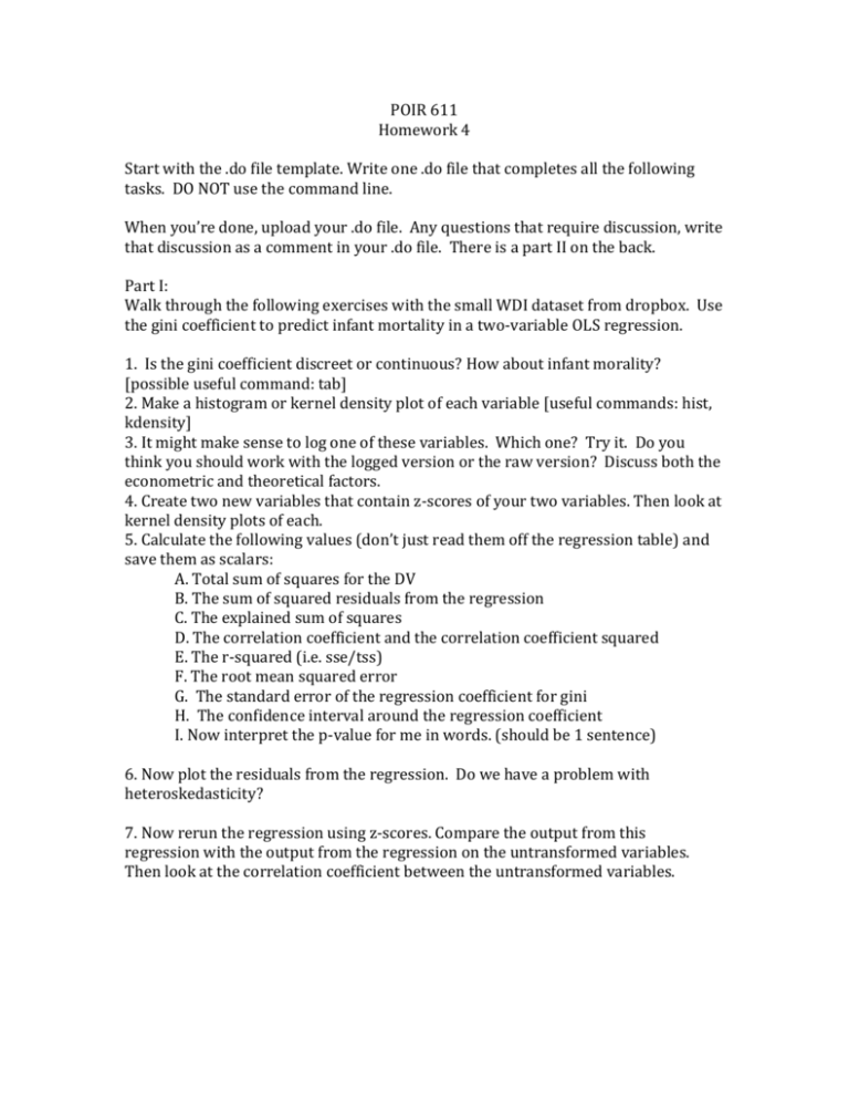
POIR 611
Homework 4
Start with the .do file template. Write one .do file that completes all the following
tasks. DO NOT use the command line.
When you’re done, upload your .do file. Any questions that require discussion, write
that discussion as a comment in your .do file. There is a part II on the back.
Part I:
Walk through the following exercises with the small WDI dataset from dropbox. Use
the gini coefficient to predict infant mortality in a two-variable OLS regression.
1. Is the gini coefficient discreet or continuous? How about infant morality?
[possible useful command: tab]
2. Make a histogram or kernel density plot of each variable [useful commands: hist,
kdensity]
3. It might make sense to log one of these variables. Which one? Try it. Do you
think you should work with the logged version or the raw version? Discuss both the
econometric and theoretical factors.
4. Create two new variables that contain z-scores of your two variables. Then look at
kernel density plots of each.
5. Calculate the following values (don’t just read them off the regression table) and
save them as scalars:
A. Total sum of squares for the DV
B. The sum of squared residuals from the regression
C. The explained sum of squares
D. The correlation coefficient and the correlation coefficient squared
E. The r-squared (i.e. sse/tss)
F. The root mean squared error
G. The standard error of the regression coefficient for gini
H. The confidence interval around the regression coefficient
I. Now interpret the p-value for me in words. (should be 1 sentence)
6. Now plot the residuals from the regression. Do we have a problem with
heteroskedasticity?
7. Now rerun the regression using z-scores. Compare the output from this
regression with the output from the regression on the untransformed variables.
Then look at the correlation coefficient between the untransformed variables.
Part II:
1. Look at kernel density plot of life expectancy. Now take the log of life expectancy.
Does it get more normal or less normal? Why?
2. Use gdppc as the DV and use the literacy rate as the IV (I know this makes less
sense theoretically than the reverse, but just go with me). Run the regression and
predict the residuals. Now make a kernel density plot of the residuals. Then a
scatterplot of the residuals and the independent variable. Now do the same thing
using ln_gdppc as the DV. How do these plots compare? Why do you think the
residuals are better behaved in one plot than the other?