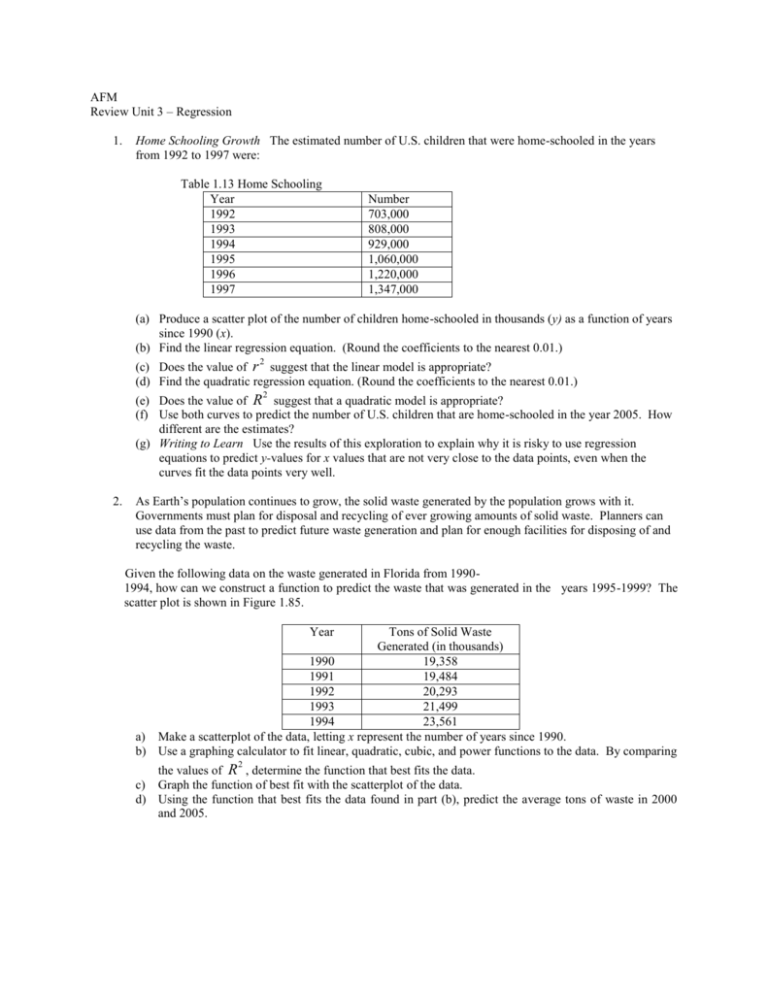
AFM
Review Unit 3 – Regression
1.
Home Schooling Growth The estimated number of U.S. children that were home-schooled in the years
from 1992 to 1997 were:
Table 1.13 Home Schooling
Year
1992
1993
1994
1995
1996
1997
Number
703,000
808,000
929,000
1,060,000
1,220,000
1,347,000
(a) Produce a scatter plot of the number of children home-schooled in thousands (y) as a function of years
since 1990 (x).
(b) Find the linear regression equation. (Round the coefficients to the nearest 0.01.)
2
(c) Does the value of r suggest that the linear model is appropriate?
(d) Find the quadratic regression equation. (Round the coefficients to the nearest 0.01.)
2
(e) Does the value of R suggest that a quadratic model is appropriate?
(f) Use both curves to predict the number of U.S. children that are home-schooled in the year 2005. How
different are the estimates?
(g) Writing to Learn Use the results of this exploration to explain why it is risky to use regression
equations to predict y-values for x values that are not very close to the data points, even when the
curves fit the data points very well.
2.
As Earth’s population continues to grow, the solid waste generated by the population grows with it.
Governments must plan for disposal and recycling of ever growing amounts of solid waste. Planners can
use data from the past to predict future waste generation and plan for enough facilities for disposing of and
recycling the waste.
Given the following data on the waste generated in Florida from 19901994, how can we construct a function to predict the waste that was generated in the years 1995-1999? The
scatter plot is shown in Figure 1.85.
Year
Tons of Solid Waste
Generated (in thousands)
1990
19,358
1991
19,484
1992
20,293
1993
21,499
1994
23,561
a) Make a scatterplot of the data, letting x represent the number of years since 1990.
b) Use a graphing calculator to fit linear, quadratic, cubic, and power functions to the data. By comparing
2
the values of R , determine the function that best fits the data.
c) Graph the function of best fit with the scatterplot of the data.
d) Using the function that best fits the data found in part (b), predict the average tons of waste in 2000
and 2005.
3.
Leisure Time The following table shows the median number of hours of leisure time that Americans had
each week in various years.
Year
1973
1980
1987
1993
1997
Source: Louis Harris and Associates
Median Number of Leisure
Hours Per Week
26.2
19.2
16.6
18.8
19.5
(a) Make a scatterplot of the data, letting x represent the number of years since 1973, and
determine which model best fits the data.
(b) Use a graphing calculator to fit the type of function determined in part (a) to the data.
(c) Graph the equation with the scatterplot. Then, use the function found in part (b) to estimate
the number of leisure hours per week in 1978,1990, and 2005.
4.
Use the data in the table below to obtain a model for speed p versus distance traveled d. Consider linear,
quadratic, exponential, and power models. Then use the model you selected as the best fit to predict the
speed of the ball at impact, given that impact occurs when d  1.80 m.
Table 2.12 Rubber Ball Data from CBR Experiment
Distance (m)
0.00000
0.04298
0.16119
0.35148
0.59394
0.89187
1.25557
5.
a)
Speed (m/s)
0.00000
0.82372
1.71163
2.45860
3.05209
3.74200
4.49558
Stopping Distance A state highway patrol safety division collected the data on stopping distances in Table
2.16.
Table 2.16 Highway Safety Division
Speed (mph)
Stopping Distance (ft)
10
15.1
20
39.9
30
75.2
40
120.5
50
175.9
Draw a scatter plot of the data.
2
b) Fit linear, quadratic, cubic, and power functions to the data. By comparing the values of R , determine the
function that best fits the data.
c) Superimpose the regression curve on the scatter plot.
d) Use the regression model to predict the stopping distance for a vehicle traveling at 25 mph.
e) Use the regression model to predict the speed of a car if the stopping distance is 300 ft.
Table 2.16 Highway Safety Division
Speed (mph)
Stopping Distance (ft)
10
15.1
20
39.9
30
75.2
40
120.5
50
175.9
6.
U.S. Farms. As the number of farms has decreased in the United States, the average size of the remaining
farms has grown larger, as shown in the table below.
Year
Average Acreage Per Farm
1910
139
1920
149
1930
157
1940
175
1950
246
1959
303
1969
390
1978
449
1987
462
1997
487
a) Make a scatterplot of the data, letting x represent the number of years since 1900.
b) Use a graphing calculator to fit linear, quadratic, cubic, and power functions to the data. By comparing
2
7.
the values of R , determine the function that best fits the data.
c) Graph the function of best fit with the scatterplot of the data.
d) Using the function that best fits the data found in part (b), predict the average acreage in 2000 and
2010.
The length of time that a planet takes to make one complete rotation around the sun is its year. The table
shows the length (in earth years) of each planet’s year and the distance of that planet from the sun (in
millions of miles). Find a model for this data in which x is the length of the year and y the distance from
the sum.
Planet
Mercury
Venus
Earth
Mars
Jupiter
Saturn
Uranus
Neptune
Pluto
8.
Year
.24
.62
1
1.88
11.86
29.46
84.01
164.79
247.69
Distance
36.0
67.2
92.9
141.6
483.6
886.7
1783.0
2794.0
3674.5
The following data was obtained by throwing a rubber ball at a CBR.
Time (sec)
0.0000
0.1080
0.2150
0.3225
0.4300
0.5375
0.6450
0.7525
0.8600
Height (m)
1.03754
1.40205
1.63806
1.77412
1.80392
1.71522
1.50942
1.21410
0.83173
a) Use the data above to make a scatterplot, letting x represent the number of seconds elapsed.
b) Next, use a graphing calculator to find the model that best expresses the height and vertical velocity of the
rubber ball. We can also use this model to predict the maximum height of the ball and its vertical velocity
when it hits the face of the CBR.
2
Fit linear, quadratic, cubic, and power functions to the data. By comparing the values of R , determine the
function that best fits the data.
d) Graph the function of best fit with the scatterplot of the data.
e) Determine the maximum height of the ball (in meters).
f) With the model you selected in part (b), predict when the height of the ball is at least 1.5 meters.
c)