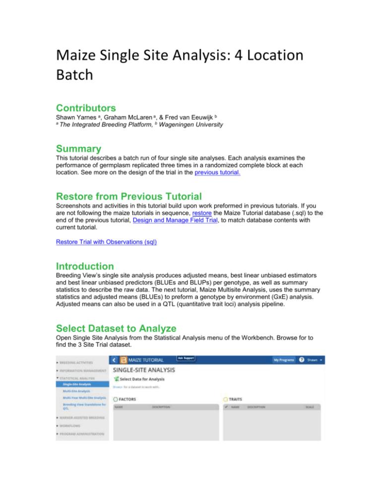
Maize Single Site Analysis: 4 Location
Batch
Contributors
Shawn Yarnes a, Graham McLaren a, & Fred van Eeuwijk b
a The Integrated Breeding Platform, b Wageningen University
Summary
This tutorial describes a batch run of four single site analyses. Each analysis examines the
performance of germplasm replicated three times in a randomized complete block at each
location. See more on the design of the trial in the previous tutorial.
Restore from Previous Tutorial
Screenshots and activities in this tutorial build upon work preformed in previous tutorials. If you
are not following the maize tutorials in sequence, restore the Maize Tutorial database (.sql) to the
end of the previous tutorial, Design and Manage Field Trial, to match database contents with
current tutorial.
Restore Trial with Observations (sql)
Introduction
Breeding View’s single site analysis produces adjusted means, best linear unbiased estimators
and best linear unbiased predictors (BLUEs and BLUPs) per genotype, as well as summary
statistics to describe the raw data. The next tutorial, Maize Multisite Analysis, uses the summary
statistics and adjusted means (BLUEs) to preform a genotype by environment (GxE) analysis.
Adjusted means can also be used in a QTL (quantitative trait loci) analysis pipeline.
Select Dataset to Analyze
Open Single Site Analysis from the Statistical Analysis menu of the Workbench. Browse for to
find the 3 Site Trial dataset.
Select the CIMMYT 2012 Trial.
Review the factors and make sure the 7 phenotypic traits measured in this trial dataset are
selected, and click Next.
Specify Analysis Conditions






Use the default analysis name.
Select Incomplete Block Design for the design type.
The factor that defines environment is LOCATION_NAME.
Select all four locations to preform individual single site analyses on each location.
REP_NO is the factor in this dataset that defines replications.
DESIGNATION defines the germplasm factor to be used in the analysis.
Click Run Breeding View to launch the breeding view application.
Run Analysis
When the Breeding View application launches the analysis conditions and data are loaded.
Notice that the four locations and all seven traits are selected with green checks. The analysis
pipeline includes a set of connected nodes, which can be used to run and configure pipelines.
Leave the default settings for the pipeline and run. Right click the first box and Run Selected
Environment Pipelines.
When the analysis is complete a popup notifies the user.
Quality Assurance
Breeding View provides an overview of potentially influential measurements to help users identify
and possibly exclude observations. Many influential observations will reflect true genotypic
variation and these data should not be excluded from the trial. The only observations that
deserve exclusion are obvious errors or measurements influenced by heterogenous
environmental variation within a block, like damage to a single plot. Select and open the Sabana
Del Medio report.
The table displays potential influential observations identified by the raw data method, which
identifies observations exceeding 1.5 times the interquartile range, and the residual method,
which identified standardized residuals by mixed model analysis. Select the potential outlier, plant
height (PH) with the value of 95.
Review the box plot for this trait as well as the related measurements for this genotype.
Exclude Observation
The measurement of 95 is well below the height measurements for other replicates of this
genotype, indicating a possible error in the phenotypic observation. Exclude this anomalous value
from the analysis by selecting Set Selected to Missing.
Re-Run Analysis
Return to the analysis pipeline and run again. Notice the boxplot for PH at Sabana Del Medio has
changed in the Quality Assurance report. The adjusted means and heritability values for this trait
will have also changed in the trial Report.
Select Upload to the BMS to save the adjusted means and summary statistics to the BMS
database for use in a subsequent genotype by environment (GxE) analysis.
Analysis Report
This section of the tutorial provides a brief guide to interpretation of the Report tab, which
includes analysis results, including graphs. The report tab summarizes the individual single
analyses preformed in batch. The majority of the results are included within the individual trial
reports.
Report Tab Contents
 Heritability Table
 Combined file of predicted means: Excel file of BLUEs and BLUPs
 Links to individual trial reports
Heritability Table
The values presented in the heritability table summarize the heritabilities calculated for each trait
by location. Broad-sense mean line heritability is derived from an estimate of the correlation
between the genotype BLUPs and their unknown true value (Cullis, Smith & Coombes, 2006). If a
model cannot be fitted to the trait data, such when there is no variability in the trait measurement,
that trait will be missing from the heritability table.
Heritability Values: Notice that some of the seven traits are missing from some or all of the
locations. For example, average shelling percentage (aSP) is missing from all locations. There
was no variation measured in this trait at any location. No adjusted means could be calculated for
this trait, because all entries were recorded as 0.788, making this trait non-informative.
Combined File of Predicted Means
Select the link to the combined file of predicted means and open in Excel. Non-informative traits
that could not be fitted with a model will appear as missing data.
BLUPs across all locations: Notice that there is no column for average shelling percentage (aSP),
because models could not be fitted to the aSP data at any location. Two traits, grain moisture
(MOI) and anthesis date (AD), at San Gilberto have empty cells for the same reason.
Individual Trial Reports
Although the four single site analyses are summarized together in the heritability table, each
location is represented by an individual analysis. Select the link to the Tlaltizapan individual trial
report to review the analysis performed at this location.
Individual trial reports include:






File of predicted means: Link to Excel (.xls) file containing an environment-specific subset
of BLUEs and BLUPs presented in the combined file of predicted means.
20 Best Genotypes Table: This table is 20 best genotypes as defined by BLUPs sorted
by the first trait. If you are interested in sorting genotypes by other traits, you can scroll
down to view the analysis of individual traits or perform a custom sort of BLUPs within the
file of predicted means (.xls).
Summary of Traits: A table presenting the minimum, mean, maximum, and heritability for
each trait within this location based on BLUPs
Estimated Genetic Correlations between traits
Principle Components Biplot
Individual Trait Analyses: Summary statistics of raw data, heritability, sorted genotype
table, summary statistics based on BLUPs, phenotypic correlations, principle components
biplot
File of Predicted Means
Tlaltizapan Report Summary: The beginning of each report provides the project name, the
environment name, the field design, and the date. Users are presented a link to the adjusted
means data for this environment, which is a subset of the data presented in the combined mean
file reporting all locations. Users are also notified about analysis failures. In this case average
shelling percentage (aSP) failed to be fitted with a mixed model, because this trait had no
reported variation within this location.
Best Genotypes Sorted by BLUPs
Tlaltizapan 20 Best Genotypes Sorted by AD: This table is the 20 best genotypes sorted by
BLUPs for the first trait, anthesis date, as defined by the default Analysis Pipeline settings under
the Generate Report node. The default settings sort values in ascending sort with large values
interpreted as “best”. So in the case of some traits, like anthesis date, where a breeder would
probably be selecting for germplasm with earlier dates, you can customize Breeding View
settings to sort by other traits, change the direction to ascending values, or sort and display the
BLUEs. You can also use the custom sort feature of Excel to sort BLUPs within the provided
spreadsheet (.xls).
Summary of Traits by BLUP
Tlaltizapan Summary of Traits: The minimum, mean, maximum, and heritability for each trait
based on BLUPs
Estimated Genetic Correlations
BLUPs Principle Components Biplot
Tlaltizapan Principle Components Biplot of BLUPs: Almost 80% of the variation observed at this
location is explained by the first two principle components. The first principle component
describes 62.42% of the variation, and is correlated most strongly to the traits: field weight (FW),
grain yield (GY), plant height (PH), and ear height (EH). The second principle component
describes 17.05% of the variation and is correlated most strongly to moisture (MOI).
Pairwise Phenotypic Correlations
Tlaltizapan Estimated Genetic Correlations: Pairwise comparison of phenotypic traits. There is a
strong positive correlation (0.9978) between the related yield measures, grain yield (GY) and field
weight (FW). These two yield traits are moderately negatively correlated (-0.6890 & -0.6830
respectively) to anthesis date. In other words, late anthesis is correlated to low yield.
Summary Statistics for Individual Trait Raw Data
Tlaltizapan Summary Statistics: Anthesis Date (AD) based on raw data
Estimated Heritability of Individual Trait
Estimated Heritability: Anthesis date (AD) calculated at Tlaltizapan
Best Genotypes by Trait Sorted by BLUEs
20 “Best” Anthesis Date (AD) Genotypes Calculated at Tlaltizapan: Genotypes are sorted by
BLUEs in descending order by value. For traits, like anthesis date, where small phenotypic
measures would be considered “best” we recommend using the custom sort features of Breeding
View under the Generate Report node or using Excel to sort BLUEs within the provided
spreadsheet (.xls).
Standard Errors of Difference
Diagnostic Bioplots of Individual Traits
Diagnostic biplots illustrate the fit of the trait data to the analysis model based on the residuals.
Residuals are estimates of experimental error obtained by subtracting the observed phenotypic
measurement from the means predicted by the model. When residuals appear to behave
randomly, it suggests that the model fits the data well. On the other hand, if non-random structure
is evident in the residuals, it suggests that the model fits the data poorly (NIST/SEMATECH eHandbook of Statistical Methods).
Well-Fitted Characteristics of Each Diagnostic Plot
 Histogram of Residuals: Gaussian, or normal, distribution
 Fitted-Value Plot: Random distribution, “shot-gun” pattern
 Normal Plot: Distribution in a straight line across the diagonal
 Half-Normal Plot: Distribution in a straight line across the diagonal
Diagnostic plots for Anthesis Data at Tlaltizapan: Example of a trait exhibiting a good model fit
Diagnostic plots for Anthesis Data at Jutiapa: Example of a trait exhibiting a poor model fit
References
Cullis, B. R., Smith, A. B., & Coombes, N. E. (2006). On the design of early generation variety
trials with correlated data. Journal of Agricultural, Biological, and Environmental Statistics, 11(4),
381-393.
Li, J., & Ji, L. (2005). Adjusting multiple testing in multilocus analyses using the eigenvalues of a
correlation matrix. Heredity, 95(3), 221-227.
Murray, D. Payne, R,, & Zhang, Z. (2014) Breeding View, a Visual Tool for Running Analytical
Pipelines: User Guide. VSN International Ltd. (.pdf) (associated sample data .zip)
NIST/SEMATECH e-Handbook of Statistical Methods, http://www.itl.nist.gov/div898/handbook/
November 2014
Funding & Acknowledgements
The Integrated Breeding Platform (IBP) is jointly funded by: the Bill and Melinda Gates
Foundation, the European Commission, United Kingdom's Department for International
Development, CGIAR, the Swiss Agency for Development and Cooperation, and the CGIAR
Fund Council. Coordinated by the Generation Challenge Program the Integrated Breeding
Platform represents a diverse group of partners; including CGIAR Centers, national agricultural
research institutes, and universities.
The statistical algorithms in the Breeding View were developed by VSNInternational Ltd in
collaboration with the Biometris group at University of Wageningen. Maize demonstration data
was provided by Mike Olsen from the CIMMYT, the International Center for Maize and Wheat
Improvement, breeding program. These data have been adapted for training purposes. Any
misrepresentation of the raw breeding data is the solely the responsibility of the IBP.
This work is licensed under a Creative Commons Attribution-ShareAlike 4.0 International License.
,