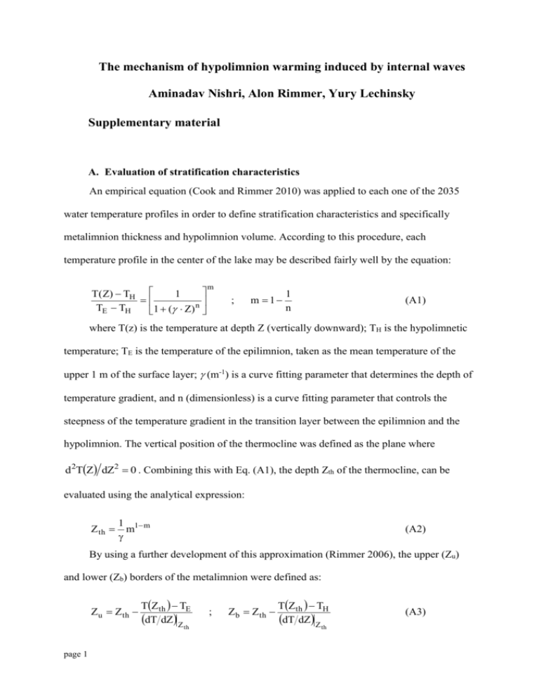
The mechanism of hypolimnion warming induced by internal waves
Aminadav Nishri, Alon Rimmer, Yury Lechinsky
Supplementary material
A. Evaluation of stratification characteristics
An empirical equation (Cook and Rimmer 2010) was applied to each one of the 2035
water temperature profiles in order to define stratification characteristics and specifically
metalimnion thickness and hypolimnion volume. According to this procedure, each
temperature profile in the center of the lake may be described fairly well by the equation:

T( Z)  TH 
1


n
TE  TH
1  (  Z) 
m
;
m 1
1
n
(A1)
where T(z) is the temperature at depth Z (vertically downward); TH is the hypolimnetic
temperature; TE is the temperature of the epilimnion, taken as the mean temperature of the
upper 1 m of the surface layer;  (m-1) is a curve fitting parameter that determines the depth of
temperature gradient, and n (dimensionless) is a curve fitting parameter that controls the
steepness of the temperature gradient in the transition layer between the epilimnion and the
hypolimnion. The vertical position of the thermocline was defined as the plane where
d 2TZ dZ2  0 . Combining this with Eq. (A1), the depth Zth of the thermocline, can be
evaluated using the analytical expression:
Z th 
1 1 m
m

(A2)
By using a further development of this approximation (Rimmer 2006), the upper (Zu)
and lower (Zb) borders of the metalimnion were defined as:
Zu  Z th 
TZ th   TE
dT dZ Z
th
page 1
;
Zb  Z th 
TZ th   TH
dT dZ Z
th
(A3)
The mechanism of hypolimnion warming
Here Zu is the thickness of the epilimnion (in meters, Fig. A1); (Zb  Zu ) is the thickness
of the metalimnion; and Z m  Z b is the thickness of the hypolimnion with Zm defined as the
maximal depth of the water body. Using the hypsographic curve of the lake V(HL) with V the
lake volume as a function of the lake absolute level HL, the epilimnion volume, VE can be
defined for every HL by:
VE  V H
L Hm
VH
L H m  Zu
.
(A4)
And the hypolimnion volume, VH can be defined for every HL by:
VH  V H
L  H m  Zb
.
(A5)
Reference:
Cook, F., & Rimmer, A. (2010). Erratum: Chemical stratification in thermally stratified lakes:
A chloride mass balance model. Limnology and oceanography, 55(3), 1463-1465.
Rimmer A, 2006. Empirical classification of stratification patterns in warm monomictic lakes.
Verh. Internat. Vertein. Limnol. 29/4: 1773-1776.
Figure A1: The empirical equation F1 applied to a water temperature profiles with =0.048
(m-1) the parameter that determines the depth of temperature gradient, and n=18.2
(dimensionless) is the parameter that controls the steepness of the temperature gradient in the
metalimnion. Here T(z) is the temperature at depth Z (vertically downward); TH is the
hypolimnetic temperature; TE is the temperature of the epilimnion.
page 2
The mechanism of hypolimnion warming
B. Hypsographic curve of Lake Kinneret
An empirical equation for the area (A, km2) and volume (V, m3) of the lake for each
absolute level, relying on VH L    AH L dH L
AH L   a  H L  e 3  b  H L  e 2  cH L  e   d
VH L   a 4  H L  e 4  b 3  H L  e 3  c 2H L  e 2  d  H L  e 
(B1)
a  0.0025; b  0.1358; c  2.6909; d  2.2249; e  255
C. water temperature profiles at 0-13 m depth in Station TH
Figures C1-C6: Continuous water temperature profiles (18 thermistors at water depth of 0.20,
0.50, 0.75, 1.00, 1.25, 1.50, 2.00 and additional 11 thermistors, 1 m apart, from depth of 3 to
13 m) at the TH monitoring station, measured with a thermistor chain (PME Temperature
Sensor with measurement accuracy of ± 0.010 °C and resolution of 0.0005 °C) on a 10
minutes time interval. Note the difference between the measured profiles as the thermocline
move downward during April to August.
page 3
The mechanism of hypolimnion warming
D. Analytical solution of T1t, z 
The seasonal temperature changes can be evaluated by solving the equation for the
annual cyclic temperature:
T1 t, z 
T 2 t, z 
 1 2
t
z
(D1)
Subject to the boundary condition:
T1 t,0  T0  TA sin  t   
(D2)
The solution is (Figure D1):

 
T1 t, z   T0  TA  exp  z 2 1 2  sin  t     z 2 1 2

(D3)
Check:

 

(D4)

 

(D5)
T1 t , z 
 TA    cos  t     z 2 1 2  exp  z 2 1 2
t
T1 t, z 
z
2

TA  

 cos  t     z 2 1 2  exp  z 2 1 2
Therefore:
T1 t, z 
T 2 t, z 
 1 2
t
z
(D6)
Figure D1: (a) Contour map of the temperature profile in the sediments until a depth of 1.5 m,
calculated from the analytical solution of the seasonal temperature, starting on day 84 of the
year (25-03-2014). (b) Simultaneous temperature measurements from SWI (0.0 m) and 1.5 m
below to the SWI, together with the analytical solution for depth of 0, 0.5, 1.0, 1.5 and 4.0
meters.
page 4
The mechanism of hypolimnion warming
E. Numerical scheme for the solution of Tt, z and Tt, z 
The equation for the short term (12 or 24) cyclic process is:
Tt, z 
T 2 t, z 

t
z 2
(E1)
Subject to the boundary condition:
Tt,0  Tt,0  T1t,0
(E2)
This problem was converted to a finite differences explicit “forward time-step” formula which
can be solved numerically:




T z j , t i 1  T z j , t i  
t
z 2
Tz j1, t i   Tz j1, t i   2Tz j , t i 
(E3)
where i = 0,1,2…Ni, and j = 0,1,2,…Nj are indexes of the time step and z depth, respectively.
The criterion for the scheme’s stability was calculated with z  2  t  (Botha and
Pinder 1983). With the given boundary condition of measured temperature T at z=0 (Eq.
D2), Eq. (D1) is solved for the first depth (z1) using:
Tz1, t i 1   Tz1, t i   
t
z 2
Tz 2 , t i   Tm z0 , t i   2Tz1, t i 
(E4)
and similarly for depth z2 and so on.
With both solutions of T and T1 the full solution is:
Tt, z  T1t, z  Tt, z
(E5)
And the heat fluxes into and out of the sediments and the exchange of the heat flux between
the sediments and the water were as follows:
q T t , z   k
Tz1, t i   Tm 0, t i 
z1
(E6)
Reference:
Botha, J. F. and G. F. Pinder. 1983. Fundamental Concepts in the Numerical Solution of
Differential Equations. John Wiley & Sons Incorporated, Hoboken, USA.
page 5
The mechanism of hypolimnion warming
F. The optimization of 
Figure F1: The modeled T(t, z) (bottom) and the measured temperatures (top), during 20 days
(10/06/2014-30/06/2014) in sediments depth of 0 to 0.3 meters.
Figure F2: Same as Figure F1 for (20/06/2014-10/07/2014).
Figure F3: The minimal root-mean-squared error (RMSE) between the measured and the
modeled temperatures were calculated for a range of  values (0.01 to 0.09 m2d-1), and the
selected  was the one with the lowest RMSE. In these two time intervals = 0.032 m2d-1 and
= 0.049 m2d-1. The optimal thermal diffusivity and the standard deviation that was reached
in the present study was 0.036 ±0.015 m2d-1.
G. Units
  k c p 
T
 2T
 2
t
z
k
T
z
c p
k


J


m  day  K 
m2



 kg   J  day

 3   
 m   kg  K 

K  m 2  K


day  day  m 2

 K
J
J
   2
 
 m  day  K  m m  day
T
J
 kg   J   K 
  
  3
  3   
t
 m   kg  K   day  m  day

  K 
J
J
   2   3
 
z
 m  day  K   m  m  day
 2T
2
J
day
W

m 2  day 86400 s m 2
page 6

(G1)
(G2)
(G3)
(G4)
(G5)
)G6)
The mechanism of hypolimnion warming
H. Empirical equation for the length of depth contours
An empirical equation for the length (L, km) of contours of the absolute level (HL, m)
was defined. It was found that:
LH L   a  H L 2  b  H L  c
;
a  0.0116 ; b  4.468 ; c  371.6 (E1)
Where a, b, and c are coefficients determined from the lake contour map, for example, L(208.9) = 55,550 m.
Figure H1: An empirical equation for the length of the contour (L, km) at the lake floor for
each absolute water level.
page 7