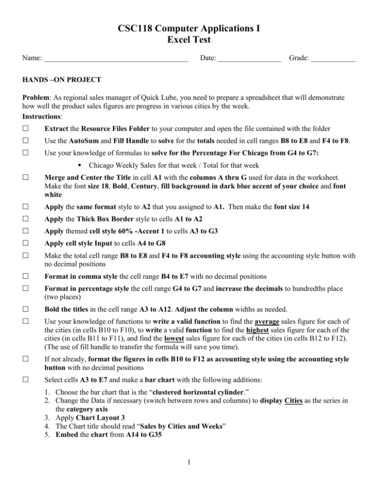
CSC118 Computer Applications I
Excel Test
Name: _______________________________________
Date: _________________
Grade: ____________
HANDS –ON PROJECT
Problem: As regional sales manager of Quick Lube, you need to prepare a spreadsheet that will demonstrate
how well the product sales figures are progress in various cities by the week.
Instructions:

Extract the Resource Files Folder to your computer and open the file contained with the folder

Use the AutoSum and Fill Handle to solve for the totals needed in cell ranges B8 to E8 and F4 to F8.

Use your knowledge of formulas to solve for the Percentage For Chicago from G4 to G7:

Chicago Weekly Sales for that week / Total for that week

Merge and Center the Title in cell A1 with the columns A thru G used for data in the worksheet.
Make the font size 18, Bold, Century, fill background in dark blue accent of your choice and font
white

Apply the same format style to A2 that you assigned to A1. Then make the font size 14

Apply the Thick Box Border style to cells A1 to A2

Apply themed cell style 60% -Accent 1 to cells A3 to G3

Apply cell style Input to cells A4 to G8

Make the total cell range B8 to E8 and F4 to F8 accounting style using the accounting style button with
no decimal positions

Format in comma style the cell range B4 to E7 with no decimal positions

Format in percentage style the cell range G4 to G7 and increase the decimals to hundredths place
(two places)

Bold the titles in the cell range A3 to A12. Adjust the column widths as needed.

Use your knowledge of functions to write a valid function to find the average sales figure for each of
the cities (in cells B10 to F10), to write a valid function to find the highest sales figure for each of the
cities (in cells B11 to F11), and find the lowest sales figure for each of the cities (in cells B12 to F12).
(The use of fill handle to transfer the formula will save you time).

If not already, format the figures in cells B10 to F12 as accounting style using the accounting style
button with no decimal positions

Select cells A3 to E7 and make a bar chart with the following additions:
1. Choose the bar chart that is the “clustered horizontal cylinder.”
2. Change the Data if necessary (switch between rows and columns) to display Cities as the series in
the category axis
3. Apply Chart Layout 3
4. The Chart title should read “Sales by Cities and Weeks”
5. Embed the chart from A14 to G35
1

Select cells range of B4 to E7 and apply a Conditional format that will make all sales figures less than
$120,000 appear red.


Name the sheet “Weekly Sales”
Then create a header and footer as stated below (be sure to use the appropriate button(s) to insert):
Header:
1. On the left should be the date and
time
2. In the Right should be the name of
the sheet




Footer
1. In the center display the page(s)
2. On the right should be your name
Change the row height of row 9 to 30 points. Re-adjust the chart if necessary so it continues to start on
cell A14 to G35.
Check spelling of the worksheet and then save the workbook file as Quick Lube- Your Name
Change the view to show the formulas version of the worksheet on one page in landscape and Save the
worksheet with the formulas showing.
Upload a copy of the workbook file to the Excel Exam section of the course
2