Chapter 10. Wind Turbine Control
[DRAFT TEXT CBPRICE 4-12-11]
[REVISED 09-12-11]
[REVISED 11-12-11]
Introduction
Energy generation by wind turbines seems to be a popular alternative source of energy for the future though
there continues to be a debate about this. At the moment Denmark produces around 20% of its energy from
wind turbines, which is actually the agreed target for the EU as a whole by 2020. The most common form of
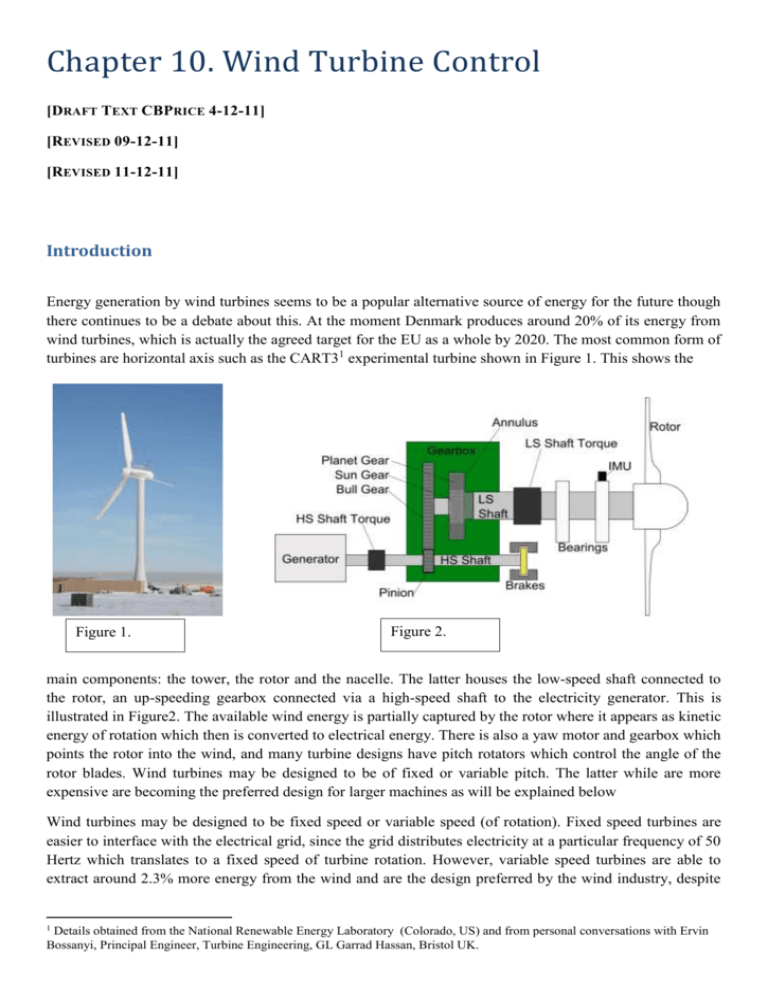
turbines are horizontal axis such as the CART31 experimental turbine shown in Figure 1. This shows the
Figure 1.
Figure 2.
main components: the tower, the rotor and the nacelle. The latter houses the low-speed shaft connected to
the rotor, an up-speeding gearbox connected via a high-speed shaft to the electricity generator. This is
illustrated in Figure2. The available wind energy is partially captured by the rotor where it appears as kinetic
energy of rotation which then is converted to electrical energy. There is also a yaw motor and gearbox which
points the rotor into the wind, and many turbine designs have pitch rotators which control the angle of the
rotor blades. Wind turbines may be designed to be of fixed or variable pitch. The latter while are more
expensive are becoming the preferred design for larger machines as will be explained below
Wind turbines may be designed to be fixed speed or variable speed (of rotation). Fixed speed turbines are
easier to interface with the electrical grid, since the grid distributes electricity at a particular frequency of 50
Hertz which translates to a fixed speed of turbine rotation. However, variable speed turbines are able to
extract around 2.3% more energy from the wind and are the design preferred by the wind industry, despite
1
Details obtained from the National Renewable Energy Laboratory (Colorado, US) and from personal conversations with Ervin
Bossanyi, Principal Engineer, Turbine Engineering, GL Garrad Hassan, Bristol UK.
requiring additional interface electronics to match the variable generator speed with the fixed grid frequency
of 50 Hertz.
Figure 3 (left) shows a graph of the power generated by the CART3 turbine as a function of wind speed
experienced. There are three clear “regions” of operation. In Region 1, the wind speed is below 2.5 m/s and
at these speeds the power generated is less than the loss of power in the machinery, so the turbine is not
allowed to rotate. In Region 2 where the wind speed is between 2.5 and 11.7 m/s the variable speed turbine
can capture more wind power than the fixed speed turbine. Finally region 3 is associated with wind speeds
from 11.7 to 20 m/s and here the power absorbed and generated is limited to the operating point to ensure
safe mechanical and electrical load limits. If the wind speed should exceed 20 m/s then the control systems
may not cope, so the turbine is shut down.
Figure 3 (right) shows two curves, the maximum power available for extraction from the wind and the actual
power which can be extracted for various wind speeds for the CART3 turbine. The latter is less than the
theoretical maximum, the reasons for this difference are explored below.
The maximum amount of power which can be absorbed from the wind is not 100% of the available wind
power, rather it is only 59% as shown by Betz [cite]. Imagine if the turbine absorbed 100% of the wind
energy, that would mean that the wind leaving the rotor would have no kinetic energy, is it would stop! This
would prevent any more wind from passing through the rotor, so this can’t happen.
Let’s start the maths by considering the power available in moving wind. Look at the volume of wind
passing through a rotor in a certain time ∆t (Figure 4). This volume is A∆l where ∆l is the length of the wind
passing through in this time. The mass of the air is mass = density x volume, i.e.,
𝜌𝐴∆𝑙
and since kinetic energy is ½ x mass x speed squared, the kinetic energy in this volume is
1
2
𝜌𝐴∆𝑙𝑣 2
but since power is energy transferred in time, for time ∆t this transfer becomes
1
2
∆𝑙
𝜌𝐴 ∆𝑡 𝑣 2
which is simply
1
2
𝜌𝐴𝑣 3
The power captured by the turbine is less than this, and depends on the individual rotor design. The
efficiency of power capture is known as the turbine’s power coefficient 𝐶𝑝 which is established by
measurement, so we finally have the following expression for the power captured
1
𝑃 = 2 𝜌𝜋𝑅 2 𝐶𝑝 𝑣 3
(1)
where R is the radius of the rotor. We shall come back to this expression later. We will need an expression
for the torque exerted on the rotor by the wind; this is obtained by dividing the power by the rotational speed
giving us
1
1
𝜏𝑅 = 2 𝜌𝜋𝑅 2 𝐶𝑝 𝑣 3 𝜔
(2)
But please remember that the power coefficient 𝐶𝑝 is not a fixed number, rather it is a function of wind
speed and turbine rotation speed.
The Turbine Controller
The controller’s job is to keep the turbine on its power curve (Figure 3). In Region 2, the controller must
ensure that the turbine extracts the maximum power from the wind given that the turbine’s rotational speed
may vary. In Region 3, the controller must ensure that the turbine extracts a fixed amount of power, even
though the available wind power may exceed this design limit. Two typical control “loops” are illustrated in
Figure 5. The “Torque” controller is used in Region 2 and it adjusts the turbine rotational speed 𝜔 to track
the wind speed v to maximize the extracted power. The “Pitch” controller is used in Region 3 and changes
the pitch of the rotor blades, so that a constant amount of power is extracted from the wind as the available
power increases with increasing wind speed.
The Torque Controller
When the wind is interacting with the rotor blades there are two speeds which are important. The first is the
speed of the wind and the second is the speed of the tip of the rotor blade. These are shown on Figure 5A.
Let’s say that the wind is blowing with a certain speed. If the rotor tip speed is larger than this then the rotor
is seen by the wind as a solid disk of obstruction since in each interval of time, the rotor is making many
revolutions while the wind is moving a small distance through it. The rotor is clearly not extracting an
optimal amount of power from the wind. On the other hand if the tip speed is small, then the rotor allows too
much wind to pass without having an impact on the turbine and again there is a sub-optimal extraction of
power. Clearly there has to be an optimal relationship between wind speed and rotor tip speed.
Each rotor design has its own optimal relationship, and this is described as a power coefficient curve which
is obtained by experiment.
Figure 5A about here.
This curve is a function of the ratio of the rotor tip speed and the wind speed. This ratio is called the “tip
speed ratio” 𝜆 and is defined as
𝜆=
𝜔𝑅
(3)
𝑣
This curve shows how the power coefficient 𝐶𝑝 but varies with 𝜆. This is plotted in Figure 6 for the CART3
turbine. The power coefficient tells you the fraction of the power which can be extracted from the wind for
various values of tip speed ratio.
𝐶𝑝
Figure 6.
𝜆
You can see here that the wind turbine operates most efficiently when the tip speed ratio is around 6. In this
case, 𝐶𝑝 is around 0.45, which means that 45% of the wind energy is being absorbed by this machine. This
compares favourably with the Betz limit of 59% mentioned above. So the turbine control systems should
adjust the tip speed ratio to be the optimal value of 6, for all operating conditions.
We can use the definition of 𝜆 to simplify the expression for the torque on the rotor produced by the wind
(see above) to
1
𝐶𝑝
𝜏𝑅 = 2 𝜌𝜋𝑅 5 𝜆3 𝜔2
(4)
Of course the rotor experiences an opposite torque provided by the generator, since the generator is
extracting energy from the rotor. Let’s call this torque 𝜏𝐺 . It is the difference between these two torques that
causes the rotor to change its rotational velocity so that it can track the changing wind velocity when it is in
Region 2. We use this difference to control the rotor speed to maximize the actual turbine 𝐶𝑝 . Also glance
back to Figure 2 where you will notice the torque sensors on the high speed and low speed shafts.
So we can write down the equation for the rate of change of rotational velocity of the rotor as
𝑑𝜔
𝑑𝑡
1
= 𝐽 (𝜏𝑅 − 𝜏𝐺 )
(5)
where J is the moment of inertia of the rotating system. This expression is the rotational equivalent of
Newton’s second law 𝑎 = 𝐹 ⁄𝑚 for translational motion. You can see that when 𝜏𝐺 = 𝜏𝐺𝑅 then the right
hand side of this expression is zero, so the rotational velocity does not increase and the rotor and wind
speeds are matched.
Now the question is how to construct an expression for 𝜏𝐺 which we can then use to control the generator
torque which will achieve an optimal extraction of wind power. This occurs at the maximum value of 𝐶𝑝 .
We need to construct an expression which when subtracted from expression (4) will give us zero. Clearly we
need 𝜏𝐺 to be proportional to 𝜔2 since it must work for all values of the rotational velocity. So we have
𝜏𝐺 = 𝐾𝜔2
and now all we have to do is choose the value of K. Well, remember this expression must look like
expression (4), so it is easy to see that there is only one possible choice for K and this is
1
𝐾 = 2 𝜌𝜋𝑅 5
𝐶𝑝𝑚𝑎𝑥
𝜆3𝑜𝑝𝑡
where 𝐶𝑝𝑚𝑎𝑥 is the maximum value of the turbine coefficient and 𝜆𝑜𝑝𝑡 is the associated “optimal” value of
the wind tip ratio. In this case expression (5) becomes
𝑑𝜔
𝑑𝑡
1
𝐶𝑝
= 2𝐽 𝜌𝜋𝑅 5 𝜔2 (𝜆3 −
𝐶𝑝𝑚𝑎𝑥
𝜆3𝑜𝑝𝑡
)
(6)
You can clearly see that when the turbine is working most efficiently where 𝐶𝑝 will have the maximum
value 𝐶𝑝𝑚𝑎𝑥 and 𝜆 will have its optimum value 𝜆𝑜𝑝𝑡 then the bracket in (6) will be zero and the rotational
velocity will not change.
The Pitch Controller
[future]
Coding the Torque Controller
omega
theta
tsr
power
Cp
Wind velocity, set by console command
or else
Rotational (angular) velocity of the rotor
Angle of the rotor at any given time
Tip speed ratio
Power generated
Power coefficient. Fraction of available
G
yep
G
G
G
G
G
yep
yep
yep
yep
yep
Default
Value
Declared?
𝜔
𝜃
𝜆
P
𝐶𝑝
Global or
Local
windV
Meaning
v
Parameter
Variable
Math
Symbol
The class provided contains a number of variables which have been declared and others which have not.
These are listed in the table below. You should use the declared variables in your code, and invent names for
those which have not been declared. Default values are also shown.
𝜏𝑅
𝜏𝐺
J
R
𝜌
𝐶𝑝𝑚𝑎𝑥
𝜆𝑜𝑝𝑡
torqueW
torqueG
error
J
R
rho
beta
CpMax
tsrOptim
vCutIn
vRated
vCutOut
omegaInit
windVInit
wind power absorbed
Torque on the rotor from the wind
Torque on the rotor from the generator
Difference between the wind and the
generator torques
Rotational inertia of the turbine
Blade radius
Density of air at the rotor height
Pitch angle of the rotor blades (not used)
Maximum value of the power coefficient
for this turbine
Value of the tip speed ratio
corresponding to the maximum value of
the power coefficient
L
L
G
no
no
yep
G
G
G
G
G
yep
yep
yep
yep
yep
G
yep 5.9
Wind speed at which the turbine becomes
operational
Wind speed at the end of Region 2.
Wind speed when the turbine is halted.
G
yep 3.1
G
G
yep 11.7
yep 20
Initial rotational velocity in the
simulation
Initial wind speed in the simulation.
G
yep 4.0
G
yep 8.0
The code template provided contains the following lines:
(1) To limit the simulation to Region 2
if(bLimitToRegionII) {
if(windV < vCutIn) windV = 0.0;
if(windV > vRated) windV = vRated;
}
(2) To calculate Cp via a look-up table
Cp = lookupPowerCoefficient(tsr,beta);
(3) To calculate the generated power
power = torqueG*omega;
You must insert additional code to compute the following:
torqueW =
torqueG =
error =
omega +=
644877
20
0.98
0.064577
0.4528
Modelling the Wind Speed
To conduct a simulation of a wind turbine response to varying wind speeds we could take two approaches.
First we could record actual wind speed changes over time and use this actual data as an input into our
simulation. This record will provide us with a distribution of wind speeds over time. While this may sound
acceptable, it is not generalizable, ie it uses just one data set and does not allow us to explore various wind
speed distributions. To conduct an investigation for various wind speed distributions, we need a model of a
generic wind speed distribution. This is the second approach.
Let’s reflect on our experience of wind speed. We can surely agree on two factors. First wind does not have
a steady speed, but it changes with time, we have gusts. Second, there are strong winds and weaker winds
(both with gusts), so we experience average wind speeds, which relate to the Beaufort scale. Therefore any
model of wind speed needs to take these two factors into account; the model should be able to represent an
average wind speed, but also to represent gusts. Since wind is complex and non-deterministic any model
must be stochastic and therefore give us information about the probability (or chance) of experiencing any
particular speed.
One good model of a wind speed distribution is the Rayleigh distribution. This tells us, given a certain
average wind speed, the chance of experiencing a variation around this average.
Have a look at Figure 7. Here the series1 blue dots show actual recorded data from a research paper2.
Analysis of the authors’ data reveals that the average wind speed is 4.81 m/s. The measured distribution of
wind speed values is interesting. It seems that there are more recorded values above the average than below.
In other words, when wind is blowing at some average speed, the gusts seem to be larger than the average. I
guess this is what we experience?
The series2 red line shows the results of the Rayleigh model which I have calculated for you. There is
reasonable agreement, not perfect, but certainly good enough to use Rayleigh’s model in our simulations,
rather than relying on actual data recorded at one time at one place.
The Rayleigh model takes as its input just one parameter, the mean (average) wind speed 𝑣𝑎𝑣 . Given this, it
predicts the chance of the wind having any other gust speed v. The expression to calculate this is as follows
𝑝(𝑣) =
2
𝜋 𝑣 −[𝜋4(𝑣𝑣 )2 ]
𝑎𝑣
𝑒
2
2 𝑣𝑎𝑣
Shimada, T., and H. Kawamura (2005), Statistical compartmentalization of surface wind field over coastal seas using high-resolution
SAR-derived winds, Geophys. Res. Lett., 32, L05607, doi:10.1029/2004GL022231
0.18
0.16
0.14
0.12
0.1
Series1
0.08
Series2
0.06
0.04
0.02
0
0
5
10
15