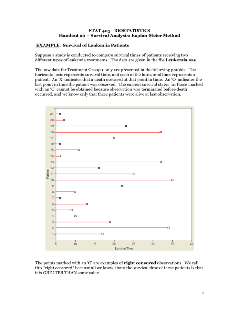
STAT 405 - BIOSTATISTICS
Handout 20 – Survival Analysis: Kaplan-Meier Method
EXAMPLE: Survival of Leukemia Patients
Suppose a study is conducted to compare survival times of patients receiving two
different types of leukemia treatments. The data are given in the file Leukemia.sas.
The raw data for Treatment Group 1 only are presented in the following graphic. The
horizontal axis represents survival time, and each of the horizontal lines represents a
patient. An ‘X’ indicates that a death occurred at that point in time. An ‘O’ indicates the
last point in time the patient was observed. The current survival status for those marked
with an ‘O’ cannot be obtained because observation was terminated before death
occurred, and we know only that these patients were alive at last observation.
The points marked with an ‘O’ are examples of right censored observations. We call
this “right censored” because all we know about the survival time of these patients is that
it is GREATER THAN some value.
1
Questions:
1. Using “conventional” statistical methods, how might you approach the analysis of
these data?
2. What are the problems with these “conventional” methods? Explain.
Survival Analysis
Conventional methods discussed earlier in the semester are not appropriate for dealing
with either censored data or time-dependent variables. In contrast, survival analysis
consists of methods for studying both the occurrence and timing of events, and these
methods allow for censoring. Several approaches to survival analysis exist, and we will
start by discussing one known as the Kaplan-Meier method.
Kaplan-Meier Method
In biostatistics, the Kaplan-Meier (KM) estimator is the most widely used method for
estimating survivor functions. When there are no censored data, the KM estimator is
simple and intuitive. For example, suppose that five patients were observed for six
months, and the following was observed:
Patient Month in Which Death Occurred
1
1
2
1
3
2
4
4
5
5
2
The survivor function, S(t), is the probability that an event time is greater than t, where t
can be any nonnegative number. In this example, an event time refers to the time at
which death occurs.
Therefore, since there is no censoring, the KM estimator Ŝ(t) is simply the sample
proportion of observations which are still alive at each time point:
i.e.
𝑆̂(𝑡) = 𝑃(𝑇 ≥ 𝑡) =
Time, t
# 𝑖𝑛𝑑𝑖𝑣𝑖𝑑𝑢𝑎𝑙𝑠 𝑤𝑖𝑡ℎ 𝑇 ≥𝑡
𝑡𝑜𝑡𝑎𝑙 𝑠𝑎𝑚𝑝𝑙𝑒 𝑠𝑖𝑧𝑒
Ŝ(t)
0
1
2
3
4
5
Kaplan-Meier estimator for censored data
When the data are censored and some of the censoring times are smaller than some
event times, the observed proportion of cases with event times greater than t can be
biased. This happens because cases that are censored before time t may have died before
time t, unbeknownst to us.
To handle this can consider using the following from conditional probability. Suppose
𝑡𝑘 < 𝑡 ≤ 𝑡𝑘+1 , then
𝑆(𝑡) = 𝑃(𝑇 ≥ 𝑡𝑘+1 ) = 𝑃(𝑇 ≥ 𝑡1 , 𝑇 ≥ 𝑡2 , … , 𝑇 ≥ 𝑡𝑘+1 )
= 𝑃(𝑇 ≥ 𝑡1 ) × ∏𝑘𝑗=1 𝑃(𝑇 ≥ 𝑡𝑘+1 |𝑇 ≥ 𝑡𝑘 )
𝑘
= ∏[1 − 𝑃(𝑇 = 𝑡𝑗 |𝑇 ≥ 𝑡𝑗 )]
𝑗=1
𝑘
= ∏[1 − 𝜆𝑗 ]
where 𝜆𝑗 = 𝑃(𝑑𝑒𝑎𝑡ℎ 𝑎𝑡 𝑡𝑖𝑚𝑒 𝑡𝑗 )
𝑗=1
3
So
𝑘
𝑆̂(𝑡) ≅ ∏ (1 −
𝑗=1
𝑑𝑗
)
𝑟𝑗
= ∏ (1 −
𝑗:𝑡𝑗 <𝑡
𝑑𝑗
)
𝑟𝑗
Here we are assuming there are k distinct event times. At each of these event times tj,
there are rj individuals who are said to be “at risk” (they have not yet experienced an
event and they have not been censored prior to time tj). Finally, we let dj be the number
who experience an event (death) at time tj and let cj denote the number of censored
observations between the j-th and (j+1)-st observed event time.
Useful identities:


𝑟𝑗 = 𝑟𝑗−1 − 𝑑𝑗−1 − 𝑐𝑗−1
𝑟𝑗 = ∑𝑘≥𝑗(𝑐𝑘 + 𝑑𝑘 )
The product derived above is called the Kaplan-Meier estimator or product-limit
estimator and is defined as:
𝑆̂(𝑡) = ∏ (1 −
𝑗:𝑡𝑗 <𝑡
𝑑𝑗
)
𝑟𝑗
EXAMPLE: Back to Survival of Leukemia Patients
For the 21 patients who received Treatment 1, the survival times of the patients are given
as follows:
6, 6, 6, 6+, 7, 9+, 10, 10+, 11+, 13, 16, 17+, 19+, 20+, 22, 23, 25+, 32+, 32+, 34+, 35+
We can use the KM method to estimate the survivor function for Treatment Group 1:
Time
tj
# at risk
nj
# of events
dj
# censored
cj
Estimated
Probability of
Surviving
 dj 
1  
 n j 
Estimated Survivor
Function
Ŝ(t) 

dj 

j

 1  n
j:t j  t
4
Using SAS for Kaplan-Meier Estimation of the Survivor Function
First, note that the data set should be constructed as follows:
data Leukemia;
input group duration censor;
datalines;
1 6 1
1 6 1
1 6 1
1 6 0
1 7 1
1 9 0
.
.
5
For each case in the data set, there must be one variable in the data set which contains
either the time that an event occurred or, for censored cases, the last time at which that
case was observed. A second variable is necessary if some of the cases are censored. It is
common to set this equal to 1 for uncensored cases and 0 for censored cases.
Specifically for our data set, the variable duration gives the time in months from the
beginning of the study to either death or censoring. The variable censor has a value of 1
for those who died and a value of 0 for those who were censored. An additional variable,
group, is an indicator variable for Treatment 1 vs. Treatment 2 patients.
To get the KM estimator, you can use PROC LIFETEST as follows:
proc lifetest data=leukemia method=km plots=(s);
where group=1;
time duration*censor(0);
symbol1 v=none;
run;
Comments regarding the ‘time’ statement:



The first variable, duration, is the time of event or censoring.
The second variable, censor, contains information on whether or not the
observation was censored.
The number in parentheses is the value of the second variable corresponding to
censored observations.
Other comments:


plots=(s) requests a plot of the survival function vs. time.
symbol1 v=none suppresses a symbol ordinarily placed at the data point on the
graph.
The output is given as follows:
6
Each of the lines in the above output corresponds to one of the 21 cases (except for the
first line, which is for time 0). Note that censored cases are marked with an asterisk.

The second column gives the KM estimator of the survivor function.

When observations share a common event or censoring time, the KM estimate is
reported for only the last case; furthermore, no estimates are reported for
censored times.

Note that although the KM estimator does not appear for all times, it is defined
for any time between 0 and the largest event or censoring time. It’s just that it
only changes at an observed event time.
Questions:
1. What is the estimated probability that a patient will survive for 16 months or
more?
2. What is the estimated survival probability for any time from 10 months up to (but
not including) 13 months?
The survivor function is graphed below:
7
SAS also returns the following:
Here, the 25th percentile refers to the smallest event time such that the probability of
dying earlier is greater than 25%. No value is reported for the 75th percentile because the
KM estimator for these data never reaches a failure probability greater than 55.18% or a
survival probability lower than 44.82%.
Note that the 50th percentile represents the median death time (here, it is 23 months).
SAS also provides an estimated mean time of death, but this estimate is biased
downward since there are censoring times greater than the largest event time. Even if
this is not the case, when a substantial number of cases are censored, the median is a
much preferred measure of central tendency for censored survival data.
Definition for Mean, Medians, and Quantiles based on the KM Estimators




Mean – ∑𝑘𝑗=1 𝑡𝑗 𝑃(𝑇 = 𝑡𝑗 )
Median – by definition, this is the time 𝜏 such that 𝑆(𝜏) = 0.5. However, in
practice, it is defined as the smallest time such that 𝑆(𝜏) ≤ 0.5. The median is
more appropriate for censored survival data than the mean.
Lower quartile – the smallest time (𝑄1 ) such that 𝑆(𝑄1 ) ≤ 0.75
Upper quartile – the smallest time (𝑄3 ) such that 𝑆(𝑄3 ) ≤ 0.25
Constructing Confidence Intervals for the KM estimators
Note that SAS also provided us with a standard error for the “survival” at each point in
time. These standard errors can be used to construct confidence intervals, which are
easily obtained using the ‘outsurv=’ option in PROC LIFETEST.
proc lifetest data=leukemia method=km outsurv=a;
where group=1;
time duration*censor(0);
run;
proc print; run;
8
̂(𝒕))
Estimating the 𝒗𝒂𝒓(𝑺
Uses the delta method which says, if Y ~𝑁(𝜇, 𝜎 2 ) then 𝑔(𝑌)is approximately normally
distributed with mean 𝑔(𝜇) and variance [𝑔′ (𝜇)]2 𝜎 2 .
For example if we consider 𝑔(𝑌) = log(𝑌) then
1 2
𝑔(𝑌)~𝑁(𝑔(𝜇), [𝑔′ (𝜇)]2 𝜎 2 ) or 𝑔(𝑌)~𝑁(log(𝜇) , (𝜇) 𝜎 2 )
and if 𝑔(𝑌) = 𝑒 𝑌 then
𝑔(𝑌)~𝑁(𝑒 𝜇 , [𝑒 𝜇 ]2 𝜎 2 )
Instead estimating the 𝑣𝑎𝑟(𝑆̂(𝑡)) we can use the delta method to approximate the
𝑣𝑎𝑟(log(𝑆̂(𝑡)). The log(𝑆̂(𝑡))=∑𝑗:𝑡 <𝑡 log(1 − 𝜆̂𝑗 ) and using independence of the 𝜆̂𝑗 ′𝑠 we
have
𝑗
𝑣𝑎𝑟[log(𝑆(𝑡))] = ∑ 𝑣𝑎𝑟[log(1 − 𝜆̂𝑗 )]
𝑗:𝑡𝑗 <𝑡
= ∑ (
𝑗:𝑡𝑗 <𝑡
1
1 − 𝜆̂𝑗
= ∑ (
𝑗:𝑡𝑗 <𝑡
= ∑
𝑗:𝑡𝑗 <𝑡
= ∑
𝑗:𝑡𝑗 <𝑡
2
) 𝑣𝑎𝑟(𝜆̂𝑗 )
1
1 − 𝜆̂𝑗
2
) 𝜆̂𝑗 (1 − 𝜆̂𝑗 )/𝑟𝑗
𝜆̂𝑗
(1 − 𝜆̂𝑗 )𝑟𝑗
𝑑𝑗
(𝑟𝑗 − 𝑑𝑗 )𝑟𝑗
9
Now 𝑆(𝑡) = exp [𝑙𝑜𝑔 (𝑆̂(𝑡))] thus by the delta method again we have
2
𝑣𝑎𝑟 (𝑆̂(𝑡)) = [𝑆̂(𝑡)] 𝑣𝑎𝑟 [log (𝑆̂(𝑡))]
thus,
𝑑𝑗
2
𝑣𝑎𝑟 (𝑆̂(𝑡)) = [𝑆̂(𝑡)] ∑
𝑗:𝑡𝑗 <𝑡
(𝑟𝑗 − 𝑑𝑗 )𝑟𝑗
This is called Greenwood’s Formula. The square root of this variance approximation
gives approximate standard errors for the estimated survivor function, i.e. 𝑆𝐸(𝑆̂(𝑡)).
Using this standard error we can compute a 95% CI for S(t) as:
𝑆̂(𝑡) ± 1.96 ∙ 𝑆𝐸[𝑆̂(𝑡)]
This can yield values outside the range [0,1]. A better approach is to exploit the delta
method even further to obtain a CI for 𝐿(𝑡) = log[− log(𝑆(𝑡))]. Since this quantity is
unrestricted, the confidence interval will be in the proper range when we transform back.
Log-log Approach for Confidence Intervals
1) Define 𝐿(𝑡) = log(− log(𝑆(𝑡)))
2) Form a 95% CI for L(t)
𝐿̂(𝑡) ± 1.96 ∙ 𝑆𝐸(𝐿̂(𝑡))
3) Since 𝑆(𝑡) = exp(− exp[𝐿(𝑡)]), the 95% CI for S(t) based on the CI for L(t) is
given by
[exp(−𝑒 (𝐿̂(𝑡)+𝐴) ) , exp(−𝑒 𝐿̂(𝑡)−𝐴 )]
4) Substituting 𝐿̂(𝑡) = log(− log (𝑆̂(𝑡))) into the upper and lower bounds gives
confidence limits
𝑒𝐴
𝑒 −𝐴
([𝑆̂(𝑡)] , [𝑆̂(𝑡)] )
10
What is 𝑆𝐸(𝐿̂(𝑡))? Using the delta method again…
2
𝑣𝑎𝑟 (𝐿̂(𝑡)) = 𝑣𝑎𝑟[𝑙𝑜𝑔(−log(𝑆̂(𝑡)))] = (
1
log (𝑆̂(𝑡))
) ∑
𝑗:𝑡𝑗 <𝑡
𝑑𝑗
(𝑟𝑗 − 𝑑𝑗 )𝑟𝑗
and the standard error is the square root of this estimated variance.
Constructing Confidence Bands for the Survivor Function
The pointwise confidence interval for the survivor function S(t) discussed above is valid
for ONLY a SINGLE FIXED TIME at which the inference is to be made. In some cases, it
is of interest to find the upper and lower confidence bands that guarantee, with a given
confidence level, that the survivor function falls within the band for all t in some interval.
One such approach was proposed by Hall and Wellner and is implemented in SAS as
follows:
ods html;
ods graphics on;
proc lifetest data=leukemia method=km outsurv=a
plots=survival(cl cb=hw);
where group=1;
time duration*censor(0);
run;
ods graphics off;
ods html close;
11
12
Testing for Differences in Survivor Functions
Now, let’s consider the observations from both treatment groups 1 and 2. To determine
whether the survivor functions differ across treatment, we test the following hypotheses:
Ho: S1(t) = S2(t) for all t
Ha: S1(t) ≠ S2(t) for all t
SAS provides three test statistics for this alternative hypothesis:
proc lifetest data=leukemia method=km plots=(s);
time duration*censor(0);
strata group;
symbol1 v=none;
symbol2 v=none;
run;
Note that the likelihood ratio statistic is calculated under the assumption that the
observations follow an exponential distribution, which is not always the case!
Also, note that SAS PROC LIFETEST returns survivor tables for both treatments (see the
table for treatment 2 below; the table for treatment 1 is the same as it was before).
13
We also obtain a plot of both survivor functions:
14
1. 00
0. 75
0. 50
0. 25
0. 00
0
5
10
15
20
25
gr oup=1
gr oup=2
30
35
dur at i on
S T RA T A :
gr oup=1
Ce n s o r e d
We can request Hall and Wellner bands for both functions by adding the ods graphics
statements and using the ‘plots’ request as shown on page 8:
plots=survival(cl cb=hw);
15
Finally, you can modify the ‘plots’ request using the ‘strata=panel’ option to specify that
separate plots for each treatment group be organized into panels instead of overlaying
them on the same plot.
plots=survival(cl cb=hw strata=panel);
16
Kaplan-Meier Estimation and Testing in R
For the 21 patients who received Treatment 1, the survival times of the patients are given
as follows: 6, 6, 6, 6+, 7, 9+, 10, 10+, 11+, 13, 16, 17+, 19+, 20+, 22, 23, 25+, 32+, 32+, 34+, 35+
[1,]
[2,]
[3,]
[4,]
[5,]
[6,]
[7,]
[8,]
[9,]
[10,]
[11,]
[12,]
[13,]
[14,]
[15,]
[16,]
[17,]
[18,]
[19,]
[20,]
[21,]
Time Censor
6
1
6
1
6
1
6
0
7
1
9
0
10
1
10
0
11
0
13
1
16
1
17
0
19
0
20
0
22
1
23
1
25
0
32
0
32
0
34
0
35
0
> fit = survfit(Surv(Time,Censor)~1,type="kaplan",conf.type="plain")
> summary(fit)
Call: survfit(formula = Surv(Time, Censor) ~ 1, type = "kaplan",
conf.type = "plain")
time n.risk n.event survival std.err lower 95% CI upper 95% CI
6
21
3
0.857 0.0764
0.707
1.000
7
17
1
0.807 0.0869
0.636
0.977
10
15
1
0.753 0.0963
0.564
0.942
13
12
1
0.690 0.1068
0.481
0.900
16
11
1
0.627 0.1141
0.404
0.851
22
7
1
0.538 0.1282
0.286
0.789
23
6
1
0.448 0.1346
0.184
0.712
> plot(fit)
> title(main="Kaplan-Meier with Greenwood-Based CI's")
17
> fit = survfit(Surv(Time,Censor)~1,type="kaplan",conf.type="log-log")
> summary(fit)
Call: survfit(formula = Surv(Time, Censor) ~ 1, type = "kaplan",
conf.type = "log-log")
time n.risk n.event survival std.err lower 95% CI upper 95% CI
6
21
3
0.857 0.0764
0.620
0.952
7
17
1
0.807 0.0869
0.563
0.923
10
15
1
0.753 0.0963
0.503
0.889
13
12
1
0.690 0.1068
0.432
0.849
16
11
1
0.627 0.1141
0.368
0.805
22
7
1
0.538 0.1282
0.268
0.747
23
6
1
0.448 0.1346
0.188
0.680
> plot(fit)
> title(main="Kaplan-Meier with Log-Log CI's")
18