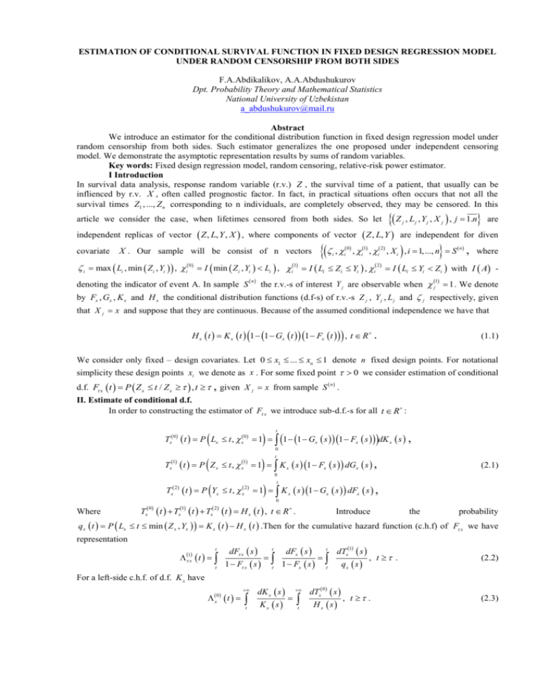
ESTIMATION OF CONDITIONAL SURVIVAL FUNCTION IN FIXED DESIGN REGRESSION MODEL
UNDER RANDOM CENSORSHIP FROM BOTH SIDES
F.A.Abdikalikov, A.A.Abdushukurov
Dpt. Probability Theory and Mathematical Statistics
National University of Uzbekistan
a_abdushukurov@mail.ru
Abstract
We introduce an estimator for the conditional distribution function in fixed design regression model under
random censorship from both sides. Such estimator generalizes the one proposed under independent censoring
model. We demonstrate the asymptotic representation results by sums of random variables.
Key words: Fixed design regression model, random censoring, relative-risk power estimator.
I Introduction
In survival data analysis, response random variable (r.v.) Z , the survival time of a patient, that usually can be
inflienced by r.v. X , often called prognostic factor. In fact, in practical situations often occurs that not all the
survival times Z1 ,..., Z n corresponding to n individuals, are completely observed, they may be censored. In this
article we consider the case, when lifetimes censored from both sides. So let
 Z , L, Y , X  ,
independent replicas of vector
covariate
where components of vector
 , 
X . Our sample will be consist of n vectors
 i  max  Li , min  Z i , Yi   , i
 0
i
 0
i
j
 Z , L, Y 
j
j
j
are
are independent for diven


, i1 , i 2 , X i , i  1,..., n  S  n , where
 I  min  Z i , Yi   Li  , i  I  Li  Zi  Yi  , i
1
denoting the indicator of event A. In sample S
 Z , L , Y , X  , j  1.n
 2
 I  Li  Yi  Zi  with I  A -
1
the r.v.-s of interest Y j are observable when  j   1 . We denote
 n
by Fx , Gx , K x and H x the conditional distribution functions (d.f-s) of r.v.-s Z j , Y j , L j and  j respectively, given
that X j  x and suppose that they are continuous. Because of the assumed conditional independence we have that


H x  t   K x  t  1  1  Gx  t   1  Fx  t   , t  R  .
(1.1)
We consider only fixed – design covariates. Let 0  x1  ...  xn  1 denote n fixed design points. For notational
simplicity these design points xi we denote as x . For some fixed point   0 we consider estimation of conditional
d.f. F x t   P  Z x  t / Z x    , t  
, given
X j  x from sample S  n  .
II. Estimate of conditional d.f.
In order to constructing the estimator of F x we introduce sub-d.f.-s for all t  R :

 
t

Tx 0  t   P Lx  t ,  x 0  1   1  1  Gx  s   1  Fx  s   dK x  s  ,
0


t
Tx1  t   P Z x  t ,  x1  1   K x  s  1  Fx  s   dGx  s  ,
(2.1)
0


t
Tx 2  t   P Yx  t ,  x 2  1   K x  s  1  Gx  s   dFx  s  ,
0
Where
Tx 0  t   Tx1  t   Tx 2  t   H x  t  , t  R  .
Introduce
the
probability
qx  t   P  Lx  t  min  Z x , Yx    K x  t   H x  t  .Then for the cumulative hazard function (c.h.f) of F x we have
representation
t
 x  t   
1

dF x  s 
t
1  F x  s 


dFx  s 
t
1  Fx  s 

dTx1  s 

qx  s 
, t  .
(2.2)
For a left-side c.h.f. of d.f. K x have
 0
x

t   
t
dK x  s 
Kx s



t
dTx 0  s 
Hx s
, t  .
(2.3)


Let  x  t   1  1  Gx  t   1  Fx  t   , Sp   x   t : 0   x  t   1 ,  mx   t   : 0  xm  t    , m  0,1 Then
a number     K x , Gx , Fx  we choose from conditions:








inf
tS p   x   ,  
K
x
 t  1   x  t    0,
(2.4)
 0
 x
1
 x  .
 - are Gasser-Müller type weights, given by
Let ni  x; hn  , i  1, n
 xn 1  x  y  
ni  x; hn    

 dy 

 0 hn  hn  
1 x
i
1  x y

 dy ,
hn  hn 

xi 1
Where x0  0,  is known density function and hn  0 as n   - sequence of bandwidths. Then the conditional
d.f.-s (1.1) and (2.1) estimated by following Stone type kernel statistics for t  R [2]:
n
H xh  t    ni  x; hn  I  i  t 
i 1
 m
Txh
 t    ni  x; hn  I  i
n
i 1
(2.5)

 m
 t , i
 1 , m  0,1, 2
By solving the integral equation (2.3) with respect to d.f. K x and using estimates (2.5) we obtain the estimator of
K x as

dTxh 0  s  

K xh  t   exp  
,t  .
 t H xh  s  
Then the probability qx  t  may be estimated by
qxh t   K xh t   H xh t  .
(2.6)
 dTxh  s 
Let 1xh  t   
, t   , is an estimate of c.h.f. (2.2). By using an ideas from [1], we introduce the
q
s


xh
t
following relative – risk power estimator of conditional survival function 1  F x  t  :
1
1  F xh
where R xh  t    xh
1
 t dq  s  
 t   xh 
  qxh  s  
 q t  
 t    xh 
 qxh   
R xh  t 
,
t 
,
(2.7)
1
III. Asymptotic representation for estimator
For investigating the estimator (2.7) we need in some notations and conditions. Let
n  min  xi  xi 1  , n  max  xi  xi 1  ,
1i  n
1i  n
and introduce the conditions
1
1
(C1) As n  , xn  1,  n  O   ,  n   n  o   ;
n
n
(C2) Kernel  have a compact support  M , M  , M  0 ,

 u   u  du  0 and 
Let
Nx t 
is Lipschitz of order 1;

is some d.f. Consider the following conditions for all
T  TN x  inf t : N x  t   1 :
 x; t   0,1  0, T 
for some
2
2
2


and
N
t
,
N
t

N
t
N
t

N x  t  exist and continuous;








x
x
x
x
xt
x 2
t 2
 sup t : H x  t   0 and  H x    T  TH x .
(C3) N x  t  
Let  H x
Theorem. Suppose that the conditions (2.4) (C1)-(C3) are hold and hn  0,
Then for all t   , T  :
n

nhn5
log n
 0,
 O 1 as n   .
nhn
log n
F xh  t   F x  t    ni  x; hn  tx   i , i  , i  , i
n
i 1
  log n 
a.s.
where sup Rn  t , x     

  nhn 
  t T

3
4
t

 txn  i , i 0 , i1 , i 2  1  F x  t   



 I 


,


i
 t, 
1
i


1
x
1 T
K x t   H x t 
t 


0
  I 

I  i   , i1  1  Tx1  
K x    H x  
i
1
2
 R
n

 s   H x  s    xh  s  dTx1  s 
 K  s   H  s 
x
t

t; x  ,
 I 
i
2

x
 s, 

1
i


 1  Tx1  s  d  K x  s   H x  s   

,
2

 K x  s   H x  s 

and
 0


  I  i  s   H x  s   dTx  s 

H x2  s 
i 1  t

n
xh  t    K x  t    
 I 


   I 


 s, i 0  1  Tx 0  s  dH x  s  



2
H x t 
Hx s
t


By using this theorem one can prove an asymptotically normality and weak convergence results for proposed
estimators(2.7).
References
i
 t , i 0  1  Tx 0  t 

i
[1] Abdushukurov A.A. Estimation of unknown distributions by incomplete observations and its properties,
LAMBERT Academic Publishing, 301 p. 2011.(In Russian).
[2] Stone C.J. Consistent nonparametric regression. //Ann. Statist. 1977. v.5. p.595-645.