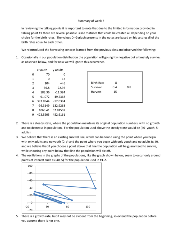
Summary of week 7
In reviewing the talking points it is important to note that due to the limited information provided in
talking point #1 there are several possible Leslie matrices that could be created all depending on your
choice for the birth rates. The values Dr Gerlach presents in the notes are based on his setting all of the
birth rates equal to each other.
We reintroduced the harvesting concept learned from the previous class and observed the following:
1. Occasionally in our population distribution the population will go slightly negative but ultimately survive,
as observed below, and for now we will ignore this occurrence.
0
1
2
3
4
5
6
7
8
9
x-youth
70
0
104
-36.8
183.36
-91.072
393.8944
-96.3149
1063.41
422.5205
y-adults
0
13
-4.6
22.92
-11.384
49.2368
-12.0394
132.9263
52.81507
452.6161
Birth Rate
Survival
Harvest
8
0.4
15
0.8
2. There is a steady state, where the population maintains its original population numbers, with no growth
and no decrease in population. For the population used above the steady state would be (40- youth, 5adults).
3. We believe that there is an existing survival line, which can be found using the point where you begin
with only adults and no youth (0, y) and the point where you begin with only youth and no adults (x, 0),
and we believe that if you choose a point above that line the population will be guaranteed to survive,
while choosing any point below that line the population will die off.
4. The oscillations in the graphs of the populations, like the graph shown below, seem to occur only around
points of interest such as (40, 5) for the population used in #1-2.
100
80
60
40
20
0
-20
-20
30
80
130
5. There is a growth rate, but it may not be evident from the beginning, so extend the population before
you assume there is not one.
The remainder of both class and the notes were based on determining the mathematics behind our
observations made in #1-5 above. In that light, when determining the steady of state of harvested
⃑⃑ can always be solved provided that
population it is important to note that the equation 𝑥⃑ = (𝐴 − 𝐼)−1 ℎ
(𝐴 − 𝐼)−1 exists, which only happens when we don’t have a singular matrix, or  = 1 is not an eigenvalue
of A. And in order to guarantee that all of the components of 𝑥⃑ are greater than zero, i.e. to guarantee
the survival of the population, we need either 𝑠1 𝑏 + 𝑠2 − 1 > 0 𝑜𝑟 𝑠1 𝑏 + 𝑠2 > 1.
We then focused on determining a general formula for calculating the eigenvalues and eigenvectors of a
harvested population, which can be seen below including several equivalent eigenvectors that can be
found using one or the other of the equations 𝑏𝑦 = 𝑥 𝑜𝑟 𝑠1 𝑥 + 𝑠2 𝑦 = 𝑦.
1 =
𝑠2 + √𝑠2 2 + 4𝑠1 𝑏
2
𝑏⁄
𝑏
[ ] , [ 1 ] , [
1
1
(1 − 𝑠2 )
 − 𝑠2
],[ 1
]
𝑠1
𝑠1
1
2 =
[
𝑠2 − √𝑠2 2 + 4𝑠1 𝑏
2
(2 − 𝑠2 )
𝑏⁄
 − 𝑠2
] , [ 2 ] , [
],[ 2
]
𝑠1
2
𝑠1
1
1
𝑏
The final topic discussed in class was the region of survival, where we looked at the vectors in two
dimensional space and their relation to the formulas we derived to represent the same phenomena.
And in the model presented in class if you let 𝑥⃑0 be the starting vector then 𝑢
⃑⃑0 = 𝑥⃑0 − 𝑥⃑ = 𝛼𝑣⃑1 + 𝛽𝑣⃑2
and it can be seen that the value for  determines whether or not the population survives or goes
extinct.