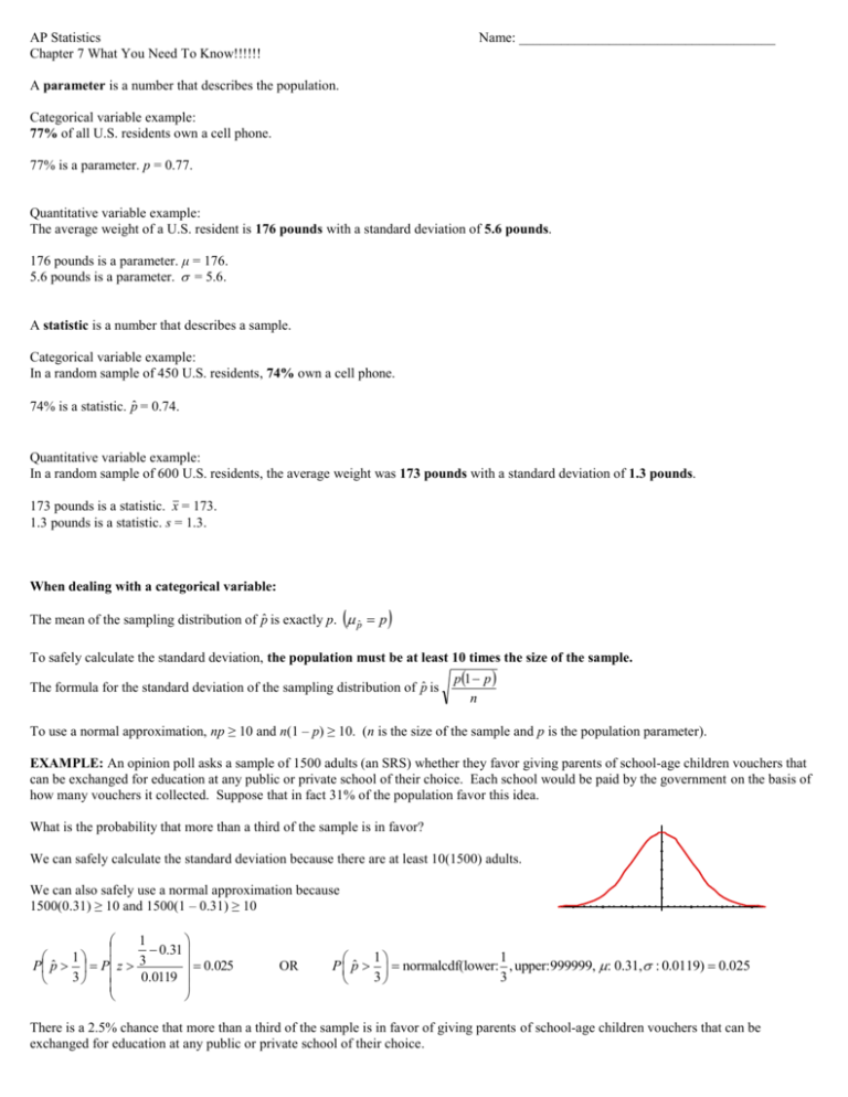
AP Statistics
Chapter 7 What You Need To Know!!!!!!
Name: _____________________________________
A parameter is a number that describes the population.
Categorical variable example:
77% of all U.S. residents own a cell phone.
77% is a parameter. p = 0.77.
Quantitative variable example:
The average weight of a U.S. resident is 176 pounds with a standard deviation of 5.6 pounds.
176 pounds is a parameter. μ = 176.
5.6 pounds is a parameter.  = 5.6.
A statistic is a number that describes a sample.
Categorical variable example:
In a random sample of 450 U.S. residents, 74% own a cell phone.
74% is a statistic. p̂ = 0.74.
Quantitative variable example:
In a random sample of 600 U.S. residents, the average weight was 173 pounds with a standard deviation of 1.3 pounds.
173 pounds is a statistic. x = 173.
1.3 pounds is a statistic. s = 1.3.
When dealing with a categorical variable:

The mean of the sampling distribution of p̂ is exactly p.  pˆ  p

To safely calculate the standard deviation, the population must be at least 10 times the size of the sample.
The formula for the standard deviation of the sampling distribution of p̂ is
p1  p 
n
To use a normal approximation, np ≥ 10 and n(1 – p) ≥ 10. (n is the size of the sample and p is the population parameter).
EXAMPLE: An opinion poll asks a sample of 1500 adults (an SRS) whether they favor giving parents of school-age children vouchers that
can be exchanged for education at any public or private school of their choice. Each school would be paid by the government on the basis of
how many vouchers it collected. Suppose that in fact 31% of the population favor this idea.
. 50
What is the probability that more than a third of the sample is in favor?
We can safely calculate the standard deviation because there are at least 10(1500) adults.
We can also safely use a normal approximation because
1500(0.31) ≥ 10 and 1500(1 – 0.31) ≥ 10
1


 0.31 

 ˆ 1
  0.025
P p    P z  3
3
0.0119 






OR
- 3. 0
3 .0
1
1

P  pˆ    normalcdf(lower: , upper:999999, : 0.31, : 0.0119)  0.025
3
3

- . 50
There is a 2.5% chance that more than a third of the sample is in favor of giving parents of school-age children vouchers that can be
exchanged for education at any public or private school of their choice.
When dealing with a quantitative variable:
The mean of the sampling distribution of x is exactly .  x   

 

The standard deviation of the sampling distribution of x is the population standard deviation divided by the square root of n.   x 

n

To safely calculate the standard deviation, the population must be at least 10 times the size of the sample.
For normality:
a) If the parent population is normally distributed, then no matter what the size of n, the sampling distribution will be approximately normal.
b) If nothing is stated about the parent population OR the parent population is not normally distributed then,
i) If n is large (≥ 30), then according to the CLT the sampling distribution will be approximately normal.
ii) If n is small, then the sampling distribution will resemble the parent population.
EXAMPLE: A certain beverage company is suspected of underfilling its cans of soft drink. The company advertises that its cans contain, on the
average, 12 ounces of soda with standard deviation 0.4 ounce.
What is the probability that a random sample of 50 cans produces a sample mean fill of 11.9 ounces or less?
The CLT allows us to assume approximate normality because n is large (n = 50).
11 .9  12 

P x  11 .9  P z 
  0.0386
0.0566 

OR
P  x  11.9  normalcdf(lower:  99999, upper:11.9, : 12, : 0.0566)  0.0386
. 50
- 3. 0
3 .0
There is a 3.86% chance that a random sample of 50 cans produces a sample mean fill of 11.9 ounces or less.
Going back to chapter 2!!!
- . 50
EXAMPLE: A certain beverage company is suspected of underfilling its cans of soft drink. The company advertises that its cans contain, on the
average, 12 ounces of soda with standard deviation 0.4 ounce. The distribution of soda cans can be considered to be approximately normally
distributed.
What is the probability that a randomly selected can is filled with 11.9 ounces or less?
11 .9  12 

Px  11 .9   P z 
  0.4013
0.4 

OR
P  x  11.9  normalcdf(lower:  99999, upper:11.9, : 12, : 0.4)  0.4013
. 50
- 3. 0
3 .0
There is a 40.13% chance that a randomly selected can is filled with 11.9 ounces or less.
- . 50