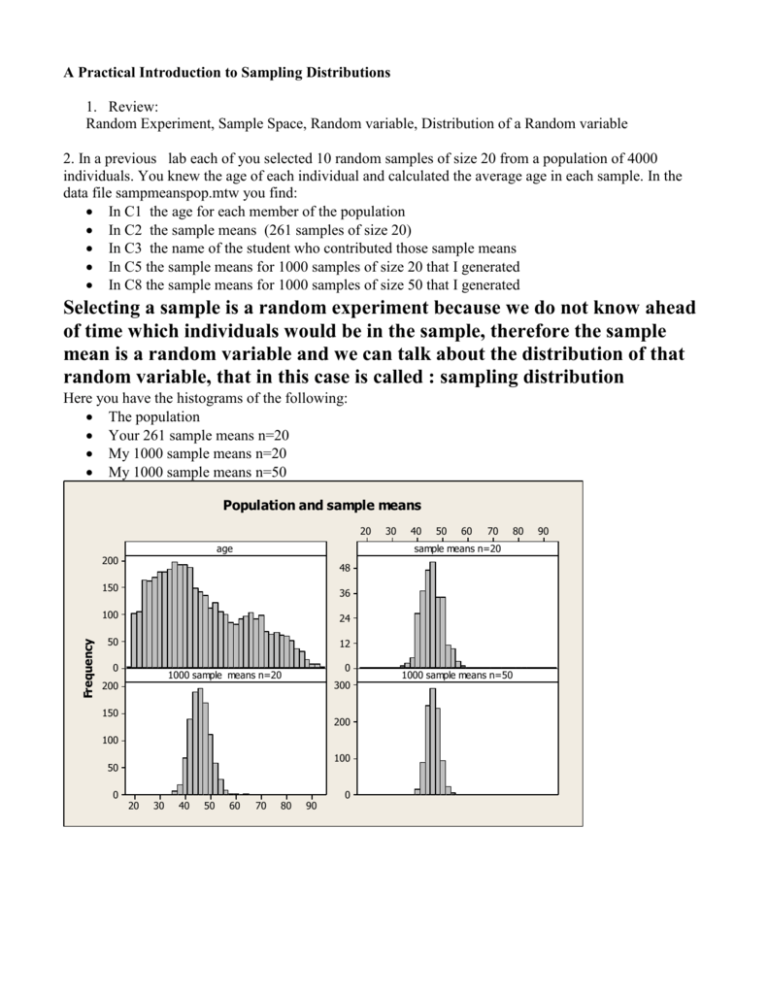
A Practical Introduction to Sampling Distributions
1. Review:
Random Experiment, Sample Space, Random variable, Distribution of a Random variable
2. In a previous lab each of you selected 10 random samples of size 20 from a population of 4000
individuals. You knew the age of each individual and calculated the average age in each sample. In the
data file sampmeanspop.mtw you find:
 In C1 the age for each member of the population
 In C2 the sample means (261 samples of size 20)
 In C3 the name of the student who contributed those sample means
 In C5 the sample means for 1000 samples of size 20 that I generated
 In C8 the sample means for 1000 samples of size 50 that I generated
Selecting a sample is a random experiment because we do not know ahead
of time which individuals would be in the sample, therefore the sample
mean is a random variable and we can talk about the distribution of that
random variable, that in this case is called : sampling distribution
Here you have the histograms of the following:
 The population
 Your 261 sample means n=20
 My 1000 sample means n=20
 My 1000 sample means n=50
Population and sample means
20
age
200
Frequency
40
50
60
70
sample means n=20
48
150
36
100
24
50
12
0
0
1000 sample means n=20
200
300
150
200
100
100
50
0
30
20
30
40
50
60
70
80
90
0
1000 sample means n=50
80
90
The mean and standard deviations are as follows
Total
Variable
Count
Mean
StDev
age
4000
45.964 17.595
sample means n=20
261
45.670
4.072
sample means n=20
1000 45.959
3.922
sample means n=50
1000 46.069
2.484
Of course if we wanted to see the ‘distribution of the sample mean for n=20 ’ we would need to take all
the possible samples of size 20 and we only have 261 samples and then 1000 samples. You can observe
the following:
 The mean of the sample means is very close to the population mean.
 The standard deviation of the sample means is smaller than the standard deviation of the
population.
 We notice that when the sample size increases the base of the histogram shrinks and the standard
deviation decreases
 The distribution of age in the population is not symmetric but the histograms of the sample means
look not only symmetric but almost normal
All those are interesting characteristics to remember. Actually when we take samples from an infinite
population (not a population of size 4000 like in our example) or if we sample with replacement, and we
consider all the possible samples of a given size, the following things are true:
(THESE 3 POINTS ARE VERY IMPORTANT TO REMEMBER)
1. About the mean: the mean of the sample means is equal to the
population mean, in math we write this as E( x )= 
2. About the standard deviation : the standard deviation of the sample
means is the standard deviation of the population divided by the square
root of the sample size  x = 
n
3. About the shape :
 If the distribution of the variable is normal the sample mean has normal
distribution regardless of sample size
 If the distribution of the variable is not normal but the sample size is
‘large enough’ the sample mean has an approximately normal distribution
(this is called the CENTRAL LIMIT THEOREM)
4. Seeing the CENTRAL LIMIT THEOREM IN ACTION
Go to the web page http://www.ruf.rice.edu/~lane/stat_sim/sampling_dist/index.html
Click on begin and you will get the following screen.
 With the mouse draw a normal distribution
 Select N=5
 click on 1,000 samples
What is the shape of the sampling distribution ?normal? It is narrower than the original
distribution? Compare the standard deviations of the population and the sample means.
 With the mouse draw a very skewed distribution
 Select N=5
 click on 1,000 samples
What is the shape of the sampling distribution? Symmetric?
Increase the sample size to N=25
Click on 1,0000 samples
Does the distribution look more symmetric? Almost normal?
The ‘large enough sample’ in the Central Limit Theorem depends of the shape of the population
or distribution of the variable. The more skewed the distribution of x is , the larger the sample
size that is needed for the distribution of x to be approximately normal.