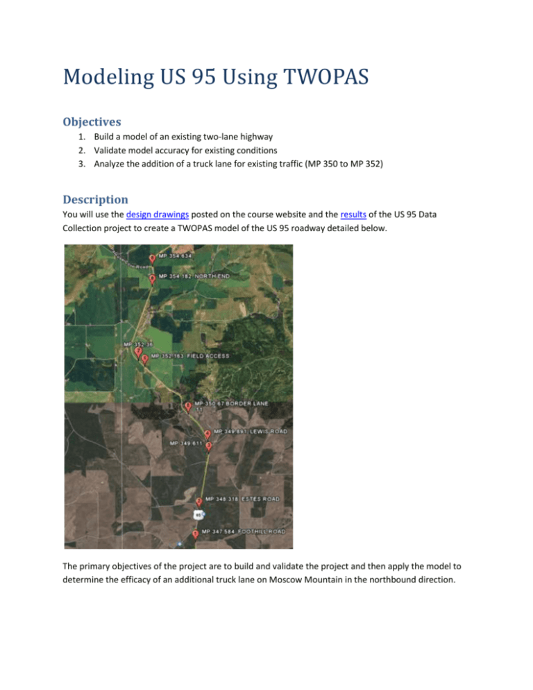
Modeling US 95 Using TWOPAS
Objectives
1. Build a model of an existing two-lane highway
2. Validate model accuracy for existing conditions
3. Analyze the addition of a truck lane for existing traffic (MP 350 to MP 352)
Description
You will use the design drawings posted on the course website and the results of the US 95 Data
Collection project to create a TWOPAS model of the US 95 roadway detailed below.
The primary objectives of the project are to build and validate the project and then apply the model to
determine the efficacy of an additional truck lane on Moscow Mountain in the northbound direction.
Building the model
Steps that you need to take to build a successful model are listed below. Refer to the TWOPAS tutorial
for instructions on each of these steps (tutorial):
1. Organize your input data as follows:
a. Aggregate volume for the entire highway section for each 10-minute time interval
b. Vehicle mix (passenger cars, RVs, and heavy trucks) by 10-minute time interval
c. Average and standard deviation of the desired travel speeds by vehicle type (combine
free flow vehicle data from all five intervals into one dataset for this measure)
d. Horizontal and vertical alignment (in design drawings)
e. Location of passing lanes/truck lanes
f. Location of revised speed limit zones (i.e., in high access locations)
g. Location of passing and no passing zones (from Google Earth)
h. List of six random number seeds, one for each replicate TWOPAS run.
i. Have a traffic data input file for each of the five time intervals.
2. Add 1-mile warm-up zones for both the northbound and southbound entry points.
3. Use 0.1 mile subsections to define the highway section. Define each TWOPAS section with the
predominant highway characteristics for the respective section in the field.
4. Have data collection stations at 0.1 mile increments, starting them after the warm-up zones and
ending them prior to the warm-up zone of the opposing direction.
5. Estimate the sight distances with UCBRURAL.
6. DON’T have UCBRURAL determine the passing and no-passing zone locations as this will likely
differ from what is in the field.
7. Make sure that you are using the correct headway threshold value. Refer to the tutorial
document for more information on checking and setting this value.
Remember that the accuracy of the highway geometry and passing zone data is limited, because they
are entered in 0.1 mile sections (i.e., it either all tangent or all curve).
Follow these steps and you are ready to run the model.
Running the model
When you run the model take the following steps:
1. Open the necessary files.
2. Let TWOPAS determine the warm-up time. It will do this for each run.
3. Input the random number seed corresponding to the replicate run you are doing (runs 1 through
6).
4. Run TWOPAS
5. Move the resulting TWOSUM.OUT file to the appropriate directory and rename it with an
informative file name.
Analyzing TWOPAS output
If you are debugging your model, then you should use UCBRURAL to view the graphs of one run in the
computer screen. Once you have reached a point where the model is producing reasonable results, you
need to make all six replicate runs and include them in your analysis. After each run, you moved and
renamed the TWOPAS.OUT file. Get the pertinent information from these files and average them for
each run scenario (i.e., traffic condition and highway characteristic). In other words, you should have six
TWOSUM.OUT files for each scenario and you should average the data that you get from these files. For
example, for interval 2 with an existing highway design, you got six values for the average travel speed
(56, 54, 60, 55, 56, and 57) from the six TWOSUM.OUT files that were output by the six runs that you
made with different random number seeds. The value that you would report is the average and
standard deviation for these average travel speed values.
Performance measures that you will use in this project are the average travel speed, the percent
following, and the number of passes. The location of these performance measures are described in the
TWOPAS tutorial.
You will analyze these measures in two forms: aggregated over the whole section and disaggregated
over each data collection station. For data in the aggregate form, report the average and confidence
interval values in tables. For the disaggregate data, you should report the station averages and
confidence interval in a graph with the measure on the y-axis and the mile post on the x-axis. See Table
1 and Figure 1 below for examples of how this should be done.
Table 1 Example Table.
Interval
1
2
3
4
5
a.
Field data
average
Simulation
Lower CIa
95% confidence interval with a sample size of 6.
90
80
percent following
70
60
50
w/o truck lane
40
w/ truck lane
30
20
10
Figure 1 Example Figure.
8.8
8.2
7
milepost
7.6
6.4
5.8
5.2
4
4.6
3.4
2.8
2.2
1
1.6
0
Upper CIa
Deliverable
Work in the groups that I have described in Table 2. I expect you to discuss your project outcomes in
seven pages or less. In your analysis, focus on answering the following questions:
1. What are the limitations of the model that exist because of input data inadequacies?
2. Does your model reflect field conditions accurately (actual values, trends)?
3. To what extent does a truck lane improve highway traffic operations? Discuss the benefits and/or
changes by vehicle type, location, and overall section.
Due December 7th at the end of the day.
Table 2 Groups
Member
Guo, Yongqing
Sekulic, Milan
Perez-Montesinos, Jean Fernando
Rahman, Mohammad Azizur
Ochoa-Huamán, Ybette Maritza
Nayak, Vidyut
Ahmed, Sk Monsur
Addei, Simon
Madrigal, Guillermo N.
Miles, Adam N
Tuly, Asma Hossain
Team
1
1
1
1
2
2
2
2
3
3
3