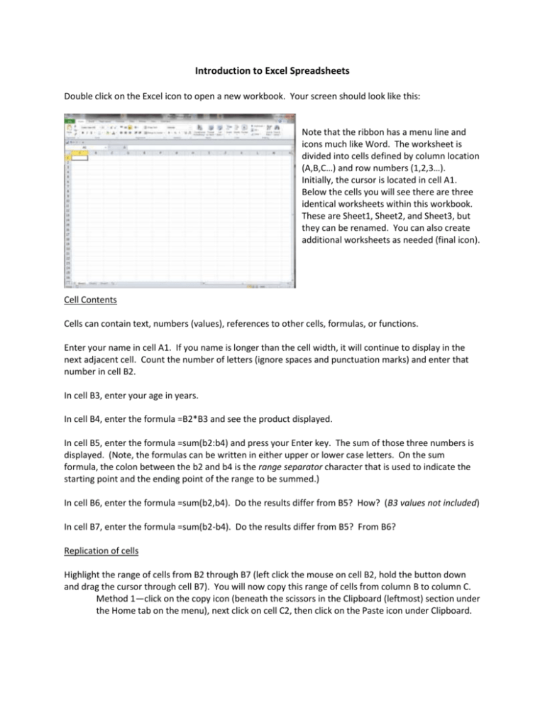
Introduction to Excel Spreadsheets
Double click on the Excel icon to open a new workbook. Your screen should look like this:
Note that the ribbon has a menu line and
icons much like Word. The worksheet is
divided into cells defined by column location
(A,B,C…) and row numbers (1,2,3…).
Initially, the cursor is located in cell A1.
Below the cells you will see there are three
identical worksheets within this workbook.
These are Sheet1, Sheet2, and Sheet3, but
they can be renamed. You can also create
additional worksheets as needed (final icon).
Cell Contents
Cells can contain text, numbers (values), references to other cells, formulas, or functions.
Enter your name in cell A1. If you name is longer than the cell width, it will continue to display in the
next adjacent cell. Count the number of letters (ignore spaces and punctuation marks) and enter that
number in cell B2.
In cell B3, enter your age in years.
In cell B4, enter the formula =B2*B3 and see the product displayed.
In cell B5, enter the formula =sum(b2:b4) and press your Enter key. The sum of those three numbers is
displayed. (Note, the formulas can be written in either upper or lower case letters. On the sum
formula, the colon between the b2 and b4 is the range separator character that is used to indicate the
starting point and the ending point of the range to be summed.)
In cell B6, enter the formula =sum(b2,b4). Do the results differ from B5? How? (B3 values not included)
In cell B7, enter the formula =sum(b2-b4). Do the results differ from B5? From B6?
Replication of cells
Highlight the range of cells from B2 through B7 (left click the mouse on cell B2, hold the button down
and drag the cursor through cell B7). You will now copy this range of cells from column B to column C.
Method 1—click on the copy icon (beneath the scissors in the Clipboard (leftmost) section under
the Home tab on the menu), next click on cell C2, then click on the Paste icon under Clipboard.
Method 2—find the small square on the bottom right corner of the frame surrounding the
selection (this is the fill square), place the cursor over it (note that the cursor changes from a fat
plus sign to a narrow one), click the left mouse button and drag it one cell to the right.
You now have two columns (B and C) displaying identical numbers in every respect. However, the
formulas in rows 4 through 7 are different. Note that all of the references to cells in column B in the
first column have now changed to references to cells in column C in the second column. You have
replicated the formulas in column B—Excel has kept the general form of the column but has changed
the references to match the new column. This differs from an exact copy of a formula.
Go to cell C2 and enter a new number that includes all characters, spaces and punctuation marks in cell
A1. Note that there is no change in cell C3, but that the others now display new values—those formulas
were dependent in one form or another on the contents of cell C2.
Go to cell A2 and enter the number corresponding to the month you were born (Jan=1, Feb=2, etc.). In
cell B8, enter the formula =b5/a2. Under the Home tab, locate the section titled Number and increase
the decimal to 3 places. Replicate this formula to column C8 and see the result—note that the formula
reads =C5/B2. What we want is to copy the formula but retain the reference to cell A2. This will involve
creating an absolute reference.
Go back to cell B8 then look at the formula display (above the cell column labels). You will see =B5/A2.
You will change this to an Absolute reference (one that does not change when the cells are copied or
replicated). Click on the cell reference on the formula display and do one of the following.
Method 1—type a dollar sign ($) before the A and before the 2 then press Enter.
Method 2—click on the A2 reference on the formula bar and press Function key #4 (F4), then
Enter.
The result will be a formula which now reads =B5/$A$2. The presence of the dollar signs transforms the
reference to an absolute reference that will not change when the cell is copied or replicated. The B5
remains a relative reference and will change to C5. Replicate the new formula from B8 to C8. Unless
values of your birth month and the number of characters in your name are equal, there should be a
change. See the differences as displayed in the two images below.
Mathematical Operators and Functions
All mathematical operations begin with the equal symbol (=).
The mathematical operators (symbols) are:
Addition:
Subtraction:
Multiplication:
Division:
Exponentiation:
+
*
/
^
(=5+2 or = B2+B3)
(=5-2 or = 17-B3)
(=5*2 or =12*12)
(=5/2 or =B9/B3)
(=5^2 or =5^.5)
A listing of functions can be accessed by either of the following methods:
Method 1—click on the fx symbol on the formula bar, then select a category and a function.
Method 2—click on the Formulas tab on the ribbon, then select one of the categories from the
Function Library.
The most frequently used categories include Financial, Logical, Text, Date and Time, Math & Trig,
Statistical, and Database.
Not all of these categories are used in this class, but a few are worthy of explanation.
Dates and Times
Excel treats dates and times as numbers. The oldest valid time is January 1, 1900 and this date has the
designated value of 1. Since dates are numbers, they can be manipulated like other numbers—they can
be added, subtracted, divided, multiplied, etc.
On your spread sheet, go to cell D1 and enter today’s date as MM/DD/YYYY or MM-DD-YYYY (actually,
only the last two digits of the year are required, and if the year is omitted then it will be assumed to be
the current year). The date will be displayed in the selected cell.
On the Home tab of the ribbon, go to the number box and see what formatting is used for cell D1 (in this
case, it should show Date. Click on the  to see additional formats. You can select to show the date as a
number (in Excel Date-Time format), or as a short date or a long date.
In cell E1, go to the Date & Time functions and select a function which automatically read today’s date
from the computer (hint: there are two possibilities—NOW and TODAY). Format that date as a number
and increase the decimals to 10 places. The number gives you the day, the decimals represent the time.
Format the cell to display the time. Note that this is a semi-static display—it is not a clock. However,
the time will change whenever the spreadsheet is recalculated.
Linking Spreadshets
In cell E3, enter the text I will be then go to cell G3 and enter the text days old on. Cell F3 will be an
input area in which you will enter a multiple of 1000 (e.g., 10,000). Cell H3 will be linked to output on a
second worksheet.
Click on the Sheet2 tab at the bottom of your workbook. This opens up an empty worksheet. Here we
will develop a template (which consists of labels, formulas, input and output areas) which will
determine on what date we will be a certain age in days. In cell A3 enter the text My birthday is: and in
A4 enter the text Age in Days: (this will be read from Sheet1). In cell B3, enter your birthday in whatever
format you choose. In cell B4, enter an equal sign ( = ), then click your cursor on the Sheet1 tab then on
cell F3, then press the Enter key.
You are returned to Sheet2 and you will see that the formula in cell B4 reads =Sheet1!F3 (meaning,
enter the contents of cell F3 from Sheet 1 here). In cell A5 of Sheet 2, enter the text On: then proceed
to cell B5. In cell B5, enter the formula =B3+B4 and press Enter. The result of this formula will appear
as either a date or a number, it really does not matter which.
Go back to Sheet1 and make a link in cell H3 to the contents of B5 on Sheet 2 (the formula will be
=Sheet2!B5). On Sheet1, format cell F3 as a number, with commas but no decimals, and format cell H3
as a date. Vary the number in cell F3 to find your next thousandth birthday. Plan on celebrating that
date with your family and/or friends.
This brief introduction to certain aspects of the spreadsheet is not an assignment. Do not submit it to
eCampus.