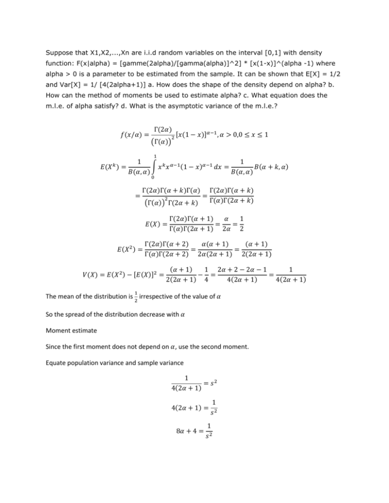
Suppose that X1,X2,...,Xn are i.i.d random variables on the interval [0,1] with density
function: F(x|alpha) = [gamme(2alpha)/[gamma(alpha)]^2] * [x(1-x)]^(alpha -1) where
alpha > 0 is a parameter to be estimated from the sample. It can be shown that E[X] = 1/2
and Var[X] = 1/ [4(2alpha+1)] a. How does the shape of the density depend on alpha? b.
How can the method of moments be used to estimate alpha? c. What equation does the
m.l.e. of alpha satisfy? d. What is the asymptotic variance of the m.l.e.?
𝑓(𝑥/𝛼) =
Г(2𝛼)
2
[𝑥(1 − 𝑥)]𝛼−1 , 𝛼 > 0,0 ≤ 𝑥 ≤ 1
(Г(𝛼))
1
1
1
𝐸(𝑋 ) =
∫ 𝑥 𝑘 𝑥 𝛼−1 (1 − 𝑥)𝛼−1 𝑑𝑥 =
𝐵(𝛼 + 𝑘, 𝛼)
𝐵(𝛼, 𝛼)
𝐵(𝛼, 𝛼)
𝑘
0
=
Г(2𝛼)Г(𝛼 + 𝑘)Г(𝛼)
2
(Г(𝛼)) Г(2𝛼 + 𝑘)
𝐸(𝑋) =
𝐸(𝑋 2 ) =
=
Г(2𝛼)Г(𝛼 + 𝑘)
Г(𝛼)Г(2𝛼 + 𝑘)
Г(2𝛼)Г(𝛼 + 1)
𝛼
1
=
=
Г(𝛼)Г(2𝛼 + 1) 2𝛼 2
(𝛼 + 1)
Г(2𝛼)Г(𝛼 + 2)
𝛼(𝛼 + 1)
=
=
Г(𝛼)Г(2𝛼 + 2) 2𝛼(2𝛼 + 1) 2(2𝛼 + 1)
𝑉(𝑋) = 𝐸(𝑋 2 ) − [𝐸(𝑋)]2 =
(𝛼 + 1)
1 2𝛼 + 2 − 2𝛼 − 1
1
− =
=
2(2𝛼 + 1) 4
4(2𝛼 + 1)
4(2𝛼 + 1)
1
The mean of the distribution is 2 irrespective of the value of 𝛼
So the spread of the distribution decrease with 𝛼
Moment estimate
Since the first moment does not depend on 𝛼, use the second moment.
Equate population variance and sample variance
1
= 𝑠2
4(2𝛼 + 1)
4(2𝛼 + 1) =
8𝛼 + 4 =
1
𝑠2
1
𝑠2
8𝛼 =
1
−4
𝑠2
𝛼=
1
1
−
2
8𝑠
2
𝛼̂ =
1
1
−
8𝑠 2 2
The moment estimate is
MLE
𝐿(𝛼) =
Г(2𝛼)
2 (∏[𝑥𝑖
(Г(𝛼))
(1 − 𝑥𝑖 )]𝛼−1 )
𝑛
𝑙𝑛(𝐿) = 𝑙𝑛(Г(2𝛼) − 2𝑙𝑛(Г(𝛼)) + (𝛼 − 1) ∑[𝑙𝑛(𝑥𝑖 ) + 𝑙𝑛(1 − 𝑥𝑖 )]
𝑖=1
𝑛
𝜕𝑙𝑛(𝐿) 𝜕𝑙𝑛(Г(2𝛼)
𝜕𝑙𝑛(Г(𝛼)
=
−2
+ ∑[𝑙𝑛(𝑥𝑖 ) + 𝑙𝑛(1 − 𝑥𝑖 )]
𝜕𝛼
𝜕𝛼
𝜕𝛼
𝑖=1
𝑛
𝜕𝑙𝑛(Г(2𝛼)
𝜕𝑙𝑛(Г(𝛼)
−2
+ ∑[𝑙𝑛(𝑥𝑖 ) + 𝑙𝑛(1 − 𝑥𝑖 )] = 0
𝜕𝛼
𝜕𝛼
𝑖=1
Or
𝑛
∑[𝑙𝑛(𝑥𝑖 ) + 𝑙𝑛(1 − 𝑥𝑖 )] = 2
𝑖=1
𝜕𝑙𝑛(Г(𝛼) 𝜕𝑙𝑛(Г(2𝛼)
−
𝜕𝛼
𝜕𝛼
is the equation to be used for finding the MLE.
Fisher information
𝐼(𝛼) = −𝐸 (
𝜕 2 𝑙𝑛(𝐿)
𝜕 2 𝑙𝑛(Г(2𝛼)
𝜕 2 𝑙𝑛(Г(𝛼)
𝜕 2 𝑙𝑛(Г(𝛼) 𝜕 2 𝑙𝑛(Г(2𝛼)
=
−𝐸
−
2
=
2
−
)
(
)
𝜕𝛼 2
𝜕𝛼 2
𝜕2𝛼
𝜕2𝛼
𝜕𝛼 2
The asymptotic variance is
1
1
=
2
𝜕 𝑙𝑛(Г(𝛼) 𝜕 2 𝑙𝑛(Г(2𝛼)
𝐼(𝛼)
2
−
𝜕2𝛼
𝜕𝛼 2
𝐿(𝛼, 𝑋1, 𝑋2, . . , 𝑋𝑛) =
Г(2𝛼)
2 (∏[𝑥𝑖
(Г(𝛼))
(1 − 𝑥𝑖 )]𝛼−1 ) =
Г(2𝛼)
2𝑡
(Г(𝛼))
𝛼−1
×1
where 𝑡 = ∏𝑛𝑖=1[𝑥𝑖 (1 − 𝑥𝑖 )]
Now the first function
Г(2𝛼)
2
(Г(𝛼))
𝑡 𝛼−1 is a function of 𝛼 and 𝑡 alone and the second function 1 is
independent of 𝛼. Therefore by Neyman’s factorization criterion, 𝑡 = ∏𝑛𝑖=1[𝑥𝑖 (1 − 𝑥𝑖 )] is a sufficient
statistic.
The MLE equation can be solved to get 𝛼 when the X1, X2, …, Xn are numerically given using tables of
digamma and trigamma functions using numerical methods or software packages. No simple formula is
possible.