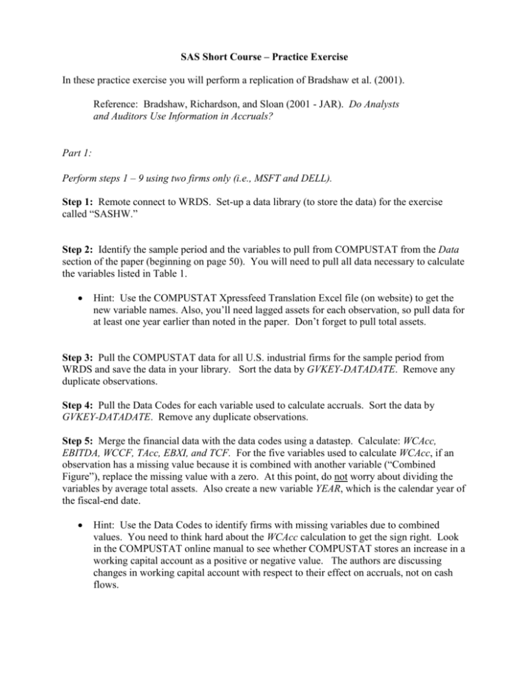
SAS Short Course – Practice Exercise
In these practice exercise you will perform a replication of Bradshaw et al. (2001).
Reference: Bradshaw, Richardson, and Sloan (2001 - JAR). Do Analysts
and Auditors Use Information in Accruals?
Part 1:
Perform steps 1 – 9 using two firms only (i.e., MSFT and DELL).
Step 1: Remote connect to WRDS. Set-up a data library (to store the data) for the exercise
called “SASHW.”
Step 2: Identify the sample period and the variables to pull from COMPUSTAT from the Data
section of the paper (beginning on page 50). You will need to pull all data necessary to calculate
the variables listed in Table 1.

Hint: Use the COMPUSTAT Xpressfeed Translation Excel file (on website) to get the
new variable names. Also, you’ll need lagged assets for each observation, so pull data for
at least one year earlier than noted in the paper. Don’t forget to pull total assets.
Step 3: Pull the COMPUSTAT data for all U.S. industrial firms for the sample period from
WRDS and save the data in your library. Sort the data by GVKEY-DATADATE. Remove any
duplicate observations.
Step 4: Pull the Data Codes for each variable used to calculate accruals. Sort the data by
GVKEY-DATADATE. Remove any duplicate observations.
Step 5: Merge the financial data with the data codes using a datastep. Calculate: WCAcc,
EBITDA, WCCF, TAcc, EBXI, and TCF. For the five variables used to calculate WCAcc, if an
observation has a missing value because it is combined with another variable (“Combined
Figure”), replace the missing value with a zero. At this point, do not worry about dividing the
variables by average total assets. Also create a new variable YEAR, which is the calendar year of
the fiscal-end date.

Hint: Use the Data Codes to identify firms with missing variables due to combined
values. You need to think hard about the WCAcc calculation to get the sign right. Look
in the COMPUSTAT online manual to see whether COMPUSTAT stores an increase in a
working capital account as a positive or negative value. The authors are discussing
changes in working capital account with respect to their effect on accruals, not on cash
flows.
Step 6: Get lagged assets and calculate total average assets for each year. Delete all
observations with invalid lags.
Step 7: Scale the earnings, cash flow, and accrual variables by average total assets.
Step 8: Delete any observation with missing earnings, cash flow, and accrual variables or any
observation outside the sample period. Only keep the firm identifiers, time identifiers, the
variables needed to create Table 1 and average assets.
Step 9: Now, re-run the code after removing the restriction for MSFT and DELL. Download
the dataset from WRDS to your machine. Save a permanent dataset.
Step 10: Using Proc Means, estimate the summary statistics in Table 1, Panel A. Create Table
1, Panel A in Excel. Include the total number of observation somewhere in the panel. Put the
variables in the same order as presented in the panel.

Don’t worry if your statistics look different than those reported in Bradshaw et al. (2001).
We haven’t made any corrections for outliers. However, the medians should be fairly
similar, as should the first and third quartiles. We have more observations than the
authors for a variety of reasons (i.e., we don’t condition of future earnings, we haven’t
removed outliers, COMPUSTAT backfills data).
Step 11: Using Proc Corr, estimate the Pearson and Spearman correlations in Table 1, Panel B.
Create Table 1, Panel B in Excel. Put the variables in the same order as presented in the panel.

Again, don’t worry if your Pearson correlations don’t line up. However, the Spearman
correlations should be similar.
Part 2:
For this assignment, we will use the database you saved at the conclusion of Part 1. However, in
order to reduce processing time, we will constrain the sample to a two-year period.
Similar to Bradshaw et al. (2001), you will be merging annual accounting data with subsequent
monthly stock return data. The following figure will help you visualize the merge for a 12/31
year-end firm.
Oct
Nov
Dec
Jan
Feb
Mar
Apr
May
Jun
Jul
Step 1: Constrain the final database you saved from Part 1 to include only those observations
with fiscal year-end dates in 1995 and 1996. Upload the data to WRDS.
Step 2: Using the COMPUSTAT / CRSP merged database in WRDS, merge in PERMNO for
each observation. Remove observations with missing PERMNOs.
Step 3: Merge in to the annual COMPUSTAT data the market data from CRSP consisting of the
monthly raw returns (RET), share volume (VOL), and shares outstanding (SHROUT). There
should be 12 monthly observations per year. The new database should consist of the following
variables: GVKEY, DATADATE, FYR, RET, VWRETD, VOL, SHROUT, & DATE.

Hint: You need stock data for the 12-month period beginning “four months after the end
of the fiscal year in which accruals are measures” (Bradshaw et al. 2001; page 56).

Hint: Assuming no stock delistments, this is a 1 to 12 merge. So, for each GVKEYDATADATE combination, you will merge in 12 months worth of stock data.
Step 4: For each month, merge in the value-weighted market return (VWRETD).
Step 5: Sort the data by GVKEY, DATADATE, DATE and remove duplicate observations.
Step 6: For each firm-year (i.e., GVKEY-DATADATE combination), calculate the cumulative
abnormal return (labeled “CAR”), the buy-and-hold abnormal return (“BHAR”), and the average
ratio of stock volume to shares outstanding (“AVOL”) over the 12-month period beginning four
months after the fiscal year-end date. Also count the number of months used in the calculations.

Hint: Try to do all of these calculations at the same time rather than in three individual
proc sql statements.
Step 7: Merge the three market variables just calculated back to the financial statement data
saved at the end of assignment two (i.e., the dataset with the accruals, cash flows, and earnings
numbers). After the merge, the new dataset should include all of the variables included in the
Part 1 dataset, plus the three market variables just calculated.
Step 8: Remove observations with missing data for any of the market variables and observations
with less than 12 months of available market data.
Step 9: Download the dataset from WRDS to your machine. Save a permanent dataset.
Step 10: Create a table (labeled Table 2, Panel A) that includes descriptive statistics for the
three market variables. The table should include the following statistics: Mean, Standard
Deviation, Median, Minimum, and Maximum, and the number of observations. Calculate the
statistics over the full time period (i.e., don’t run the statistics separately for each year).
Part 3:
Step 1: Pull in the dataset you saved at the end of Part 1.
Step 2: Winsorize the following accounting variables at the top and bottom 0.5% of the
distribution by year: EBXI, TCF, EBITDA, TAcc, WCAcc, & WCCF.

Hint: After you winsorize the variables, drop the percentile cut-point data from the
dataset.
Step 3: Create a table (labeled Table 3, Panel A) that includes the Mean and Std Dev. for the six
earnings, cash flow, and accrual variables. Compare this mean to Table 1, Panel A in Bradshaw
et al. (2001) and to the mean you calculated back in assignment 2.

Note: The statistics are much closer now to those reported in Bradshaw et al. (2001).
Step 4: Now, pull in the dataset you saved at the end of Part 2. Trim (throw out) the following
accounting variables at the top and bottom 1% of the distribution by year: TAcc & WCAcc.
Step 5: Using pooled OLS, estimate the following model and create a table (labeled Table 3,
Panel B) that reports the following: variables, coefficient estimates, t-stats, R2, and the number
of observations.
BHAR = β0 + β1 WCAcc + β2 WCCF + ε
Step 6: Repeat step 5, but adjust the standard errors for heteroskedasticity and cross-sectional
correlation in the error terms (i.e., cluster on year). Report the results in Panel C.

Compare the OLS and adjusted results.