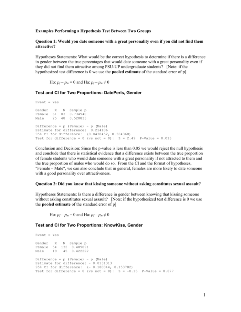
Examples Performing a Hypothesis Test Between Two Groups
Question 1: Would you date someone with a great personality even if you did not find them
attractive?
Hypotheses Statements: What would be the correct hypothesis to determine if there is a difference
in gender between the true percentages that would date someone with a great personality even if
they did not find them attractive among PSU-UP undergraduate students? [Note: if the
hypothesized test difference is 0 we use the pooled estimate of the standard error of p]
Ho: pf – pm = 0 and Ha: pf – pm ≠ 0
Test and CI for Two Proportions: DatePerls, Gender
Event = Yes
Gender
Female
Male
X
61
25
N
83
48
Sample p
0.734940
0.520833
Difference = p (Female) - p (Male)
Estimate for difference: 0.214106
95% CI for difference: (0.0438452, 0.384368)
Test for difference = 0 (vs not = 0): Z = 2.49
P-Value = 0.013
Conclusion and Decision: Since the p-value is less than 0.05 we would reject the null hypothesis
and conclude that there is statistical evidence that a difference exists between the true proportion
of female students who would date someone with a great personality if not attracted to them and
the true proportion of males who would do so. From the CI and the format of hypotheses,
"Female – Male", we can also conclude that in general, females are more likely to date someone
with a good personality over attractiveness.
Question 2: Did you know that kissing someone without asking constitutes sexual assault?
Hypotheses Statements: Is there a difference in gender between knowing that kissing someone
without asking constitutes sexual assault? [Note: if the hypothesized test difference is 0 we use
the pooled estimate of the standard error of p]
Ho: pf – pm = 0 and Ha: pf – pm ≠ 0
Test and CI for Two Proportions: KnowKiss, Gender
Event = Yes
Gender
Female
Male
X
54
19
N Sample p
132 0.409091
45 0.422222
Difference = p (Female) - p (Male)
Estimate for difference: - 0.0131313
95% CI for difference: (- 0.180044, 0.153782)
Test for difference = 0 (vs not = 0): Z = -0.15
P-Value = 0.877
1
Conclusion and Decision: Since the p-value is greater than 0.05 we would fail to reject the null
hypothesis and conclude that there is no statistical evidence to conclude a difference exists
between the genders in the proportion who know that kissing without asking constitutes sexual
assault.
Question 2: How much are you willing to spend on a first date?
Ho: uf − um = 0 and Ha: uf − um ≠ 0
Before we proceed we need to address a new concept related to the standard error. When we
consider comparing two or more populations it would be helpful if we could assume that the
variability of each population is the same even if the means differ. The general rule of thumb to
determine equal variances for two populations is to compare the two sample standard deviations.
If the ratio of the larger to the smaller is less than or equal to 2.0 we can assume the variances are
equal. This looks like the following:
S larger
Ssmaller
 2.0
Using descriptive statistics, the larger S is 69.9 (male) and 18.5 (female) is the smaller. The ratio
then is 69.9/18.5 > 2.0 thus we can assume the variances for the female and male populations are
NOT equal. With the variances assumed equal, we use the unpooled method in calculating our
standard error.
S.E.(unpooled) =
S +S
2
2
1
2
N1
N2
2
=
69.9 + 18.5
45
131
2
=10.54
If the variances are assumed equal, we use:
S.E.(pooled) = S p
1
1
where Sp =

N1 N 2
( N1  1) * S12  ( N 2  1) * S22
N1  N 2  2
A 95% confidence interval for the true difference would equal:
(X-barf -X-barm) +/- 1.96*2.64 = (42.8 – 51.9) +/- 2*10.54 = -9.1 +/- 21.08 = -30.18, 11.98
Two-Sample T-Test and CI: DateSpnd, Gender
Two-sample T for DateSpnd
Gender
female
male
N
131
45
Mean
42.8
51.9
StDev
18.5
69.9
SE Mean
1.6
10
Difference = mu (female) - mu (male)
Estimate for difference: -9.0
95% CI for difference: (-30.3, 12.2)
T-Test of difference = 0 (vs not =): T-Value = -0.86
P-Value = 0.396
DF = 46
2
Conclusion and Decision: Since the p-value is greater than 0.05 we would fail to reject the null
hypothesis and conclude that there is no difference between the genders in the mean amount of
money spent on a date. Also, since we the confidence interval for the mean difference includes
zero, this would further support our decision to not conclude a difference in means exist.
Question 4: Is there a difference in car estimates between two repair shops?
We could either treat the samples as two independent samples and conduct a two-mean test, OR
we can conduct a test that compares across the shops i.e. compares the estimates of the two shops
on the same car.
Ho: u1 – u2 = 0 and Ha: u1 – u2 ≠ 0
Two-Sample T-Test and CI: One, Two
Two-sample T for One vs Two
Pre_87
No
Yes
N
15
15
Mean
16.83
16.23
StDev
3.22
2.94
SE Mean
0.83
0.76
Difference = mu (One) - mu (Two)
Estimate for difference: 0.59
95% CI for difference: (-1.71, 2.90)
T-Test of difference = 0 (vs not =): T-Value = 0.53 P-Value = 0.602 DF = 28
Both use Pooled StDev = 3.0830 NOTE- See if you can calculate this value by
hand using the steps outlined in Question 2
With p-value 0.602 we would fail to reject Ho and conclude that there is no difference in mean
repair costs between the two shops. Also, with the 95% CI including zero this would further
support that there is no difference in average repair estimates between the two shops.
Ho: ud = 0 and Ha: ud ≠ 0 where the difference is found by taking Shop One estimates minus
Shop Two estimates
Paired T-Test and CI: One, Two
Paired T for One - Two
One
Two
Difference
N
15
15
15
Mean StDev SE Mean
16.827 3.219
0.831
16.233 2.941
0.759
0.593 0.403
0.104
95% CI for mean difference: (0.370, 0.816)
T-Test of mean difference = 0 (vs not = 0): T-Value = 5.71
P-Value = 0.000
With p-value 0.000 we would reject Ho and conclude that there is a difference in mean repair
costs between the two shops. Also, with the 95% CI being positive and the difference found by
taking the One minus Two, we conclude that on average Shop One charges statistically
significantly more for estimates than Shop Two.
3