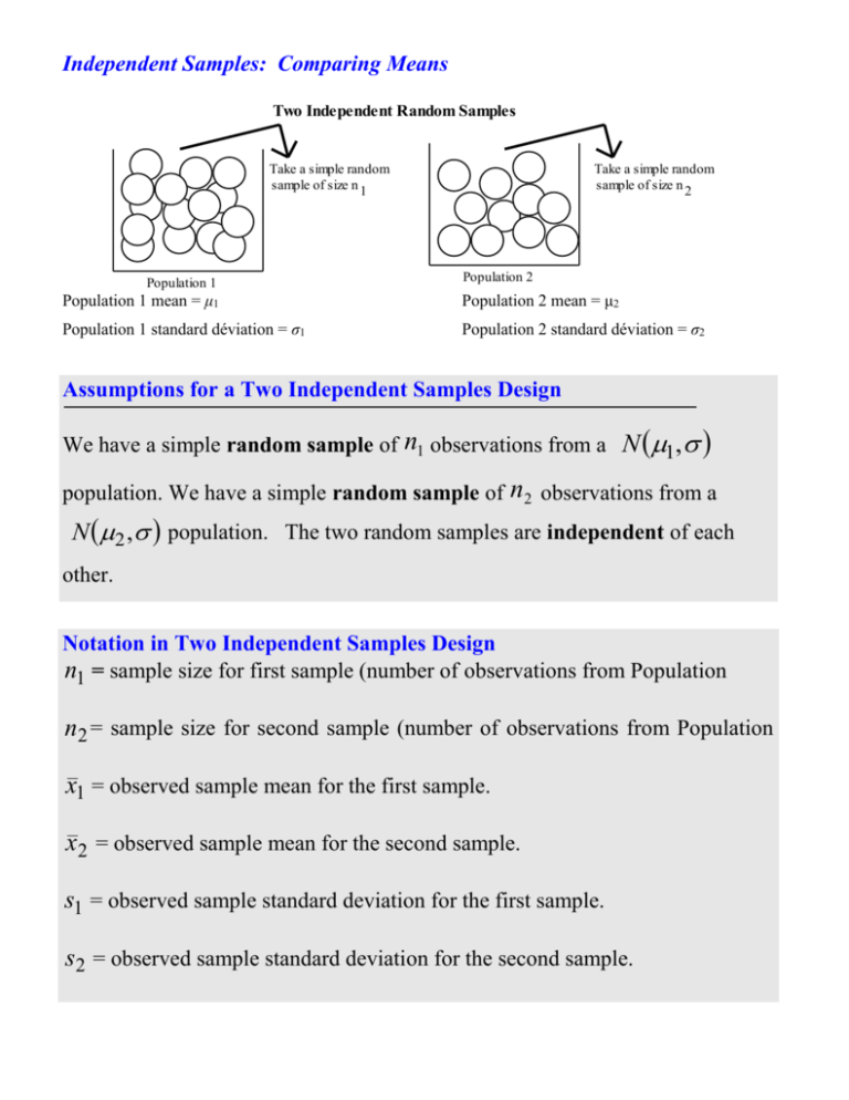
Independent Samples: Comparing Means
Two Independent Random Samples
Take a simple random
sample of size n 1
Population 1
Take a simple random
sample of size n 2
Population 2
Population 1 mean = μ1
Population 2 mean = μ2
Population 1 standard déviation = σ1
Population 2 standard déviation = σ2
Assumptions for a Two Independent Samples Design
We have a simple random sample of
n1 observations from a N 1, 
population. We have a simple random sample of
n2 observations from a
N 2 ,  population. The two random samples are independent of each
other.
Notation in Two Independent Samples Design
n1 = sample size for first sample (number of observations from Population
n2 = sample size for second sample (number of observations from Population
x1 = observed sample mean for the first sample.
x2 = observed sample mean for the second sample.
s1 = observed sample standard deviation for the first sample.
s2 = observed sample standard deviation for the second sample.
Testing the Difference Between Two Means of Independent Samples Design
There are actually two different options for the use of t tests. One
option is used when the variances of the populations are not equal, and
the other option is used when the variances are equal. To determine
whether two sample variances are equal, the researcher
can use an F test.
Note, however, that not all statisticians are in agreement about using
the F test before using the t test. Some believe that conducting the F
and t tests at the same level of significance will change the overall level
of significance of the t test. Their reasons are beyond the scope of this
course.
Assumptions:
- Both populations are normally distributed
-The samples are obtained independently
Not satisfied
Non-parametric
method are used
TEST if the variances of two
normally distributed
populations
Satisfied
are different
H 0 :  12   22
H1 :  12   22
Using F-test
Did not reject
Reject
Pooled T-test
H 0 : 1   2
To test
To test
H1 : 1   2
Use the test statistic
T 
X
1
sp
 X2

d0
1
1

n1
n2
Where
sp 
Non-pooled T-test
n1  1s12  n2  1s22
n1  n2  2
H 0 : 1   2
H1 : 1   2
Use the test statistic
( x  x )  ( 1  2 )
t 1 2
s12 s22

n1 n2
With approximate d.f.
2
 s12
s22 



n2 
 n1
df 
2
2
 s12 
 s22 




 n1    n2 
n1  1
n2  1
Let’s Do It! 1
Which Version of a Two Independent Samples Test to Use?
Each scenario presents a picture of the distributions of the two
populations being compared. Based on these distributions, determine
which version of the two-independent samples test to use.
Version of Test:
(select one)
Pooled t-test
Nonpooled t-test
Nonparametric test
Explain:
Version of Test:
Pooled t-test
Nonpooled t-test
Nonparametric test
Explain:
Version of Test:
(select one)
Explain:
Pooled t-test
Nonpooled t-test
Nonparametric test
Two Independent Samples Pooled t-Test
We are interested in comparing the population means 1
parameter of interest is the difference 1   2 .
and  2 , so the
Distribution of the Standardized X 1  X 2 for the Two Independent
Samples Scenario when  1   2
The quantity
Where sp 
T 
X
1
sp

 X 2  d0
1
1

n1 n2
n1  1s12  n2  1s22
, has a t-distribution with
n1  n2  2
n1  n2  2
degrees of freedom.
Two Independent Samples Pooled t-Test
Assumptions:
The first sample is a random sample from a normal
population with mean  1. The second sample is a random sample from
a normal population with mean  2. The two samples are independent.
Normality is less crucial if the sample sizes n1 and n2 are large,
Hypotheses: H0 : 1   2  d0 versus H1 : 1   2  d0 or
versus
H1 : 1  2  d or
versus H1 : 1  2  d .
Data:
The two sets of data from which the two sample means x1
and x 2 , and the two sample standard deviations s1 and s 2 can
be computed.
x1  x 2  d 0
(n1  1) s12  (n2  1) s 22
Observed Test Statistic: t 
where s p 
n1  n2  2
1
1
sp
n1

n2
And the t-distribution used has d.f.= (n1+ n2 – 2)
p-value:
We find the p-value for the test using the t(n1+ n2 - 2)
distribution. The direction of extreme will depend on how the
alternative hypothesis is expressed.
EXAMPLE
Comparing Two Headache Treatments
Medical researchers are comparing two treatments for
migraine headaches. They wish to perform a doubleblind experiment to assess if Treatment B (the new
treatment) is significantly better than Treatment A (the standard
treatment) using a 5% significance level. Assume equal variances of the
populations. The data
nA  10 x A  19.4 s A  4.9
nB  10 x B  22.6 sB  5.2
(a)
State the appropriate hypotheses to be tested. Keep in mind that
smaller responses imply a better treatment and Treatment 1 is the
new treatment.
H0 :  B   A  0 vs H1 :  B   A  0
(b) Give an estimate of the common (pooled) population standard
deviation.
sp 
(c)
10  1 5.2 2  10  1 4.9 2
10  10  2
 5.05
Compute the pooled t-test statistic.
t 
22.6  19.4
5.05
 1.416
1
1

10 10
(d) Find the corresponding p-value.
The p-value is the probability of observing a test statistic as large as or
larger than the observed value of 1.416, with d.f= 10 +10 -2 =18
Using the TI:
1.
Using the tcdf( function.
Using the tcdf( function on the TI we have:
p-value = P T  1.416= tcdf(1.416, E99, 18) =
0.0869.
t(18)
Area=p-value
0
1.416
2.
Using the 2-SampTTest function under STAT TESTS.
In the TESTS menu located under the STAT button, we select the 4:2SampTTest option. With the sample means of 22.6 and 19.4, the
sample standard deviations of 5.2 and 4.9, and the sample sizes of 10
and 10, we can use the Stats option of this test. The steps and
corresponding input and output screens are shown. Notice that you
must specify Yes under the Pooled option. The No Pooled option is
discussed at the end of this section as another version of our test.
p-value = P T  1.416= 0.08688.
(g)
State the decision and conclusion using a 5%significance level.
At the 5% significance level we cannot reject the null hypothesis.
The samples failed to provide any significant results.
Let’s Do It!
Drug 1
Drug 2
Sample
Size
12
14
Sample Mean
5.6
5.0
Sample Standard
Deviation
1.3
1.8
(a)
Assume the two equal population variances and the assumption of
independent samples is satisfied. Suppose we can assume each
sample is representative of the larger population of potential drug
users. One more assumption is required regarding the populations.
What is that assumption?
(d)
Is the difference between the mean cholesterol reduction for Drug
1 and the mean cholesterol reduction for Drug 2 statistically
significant at the 5% level?
Hypothesis:
Test statistic:
P-value:
Decision:
Conclusion:
Homework Page339: 11, 12, 13, 29, 30, 40, 47 (assume
variances are equal for all problem)