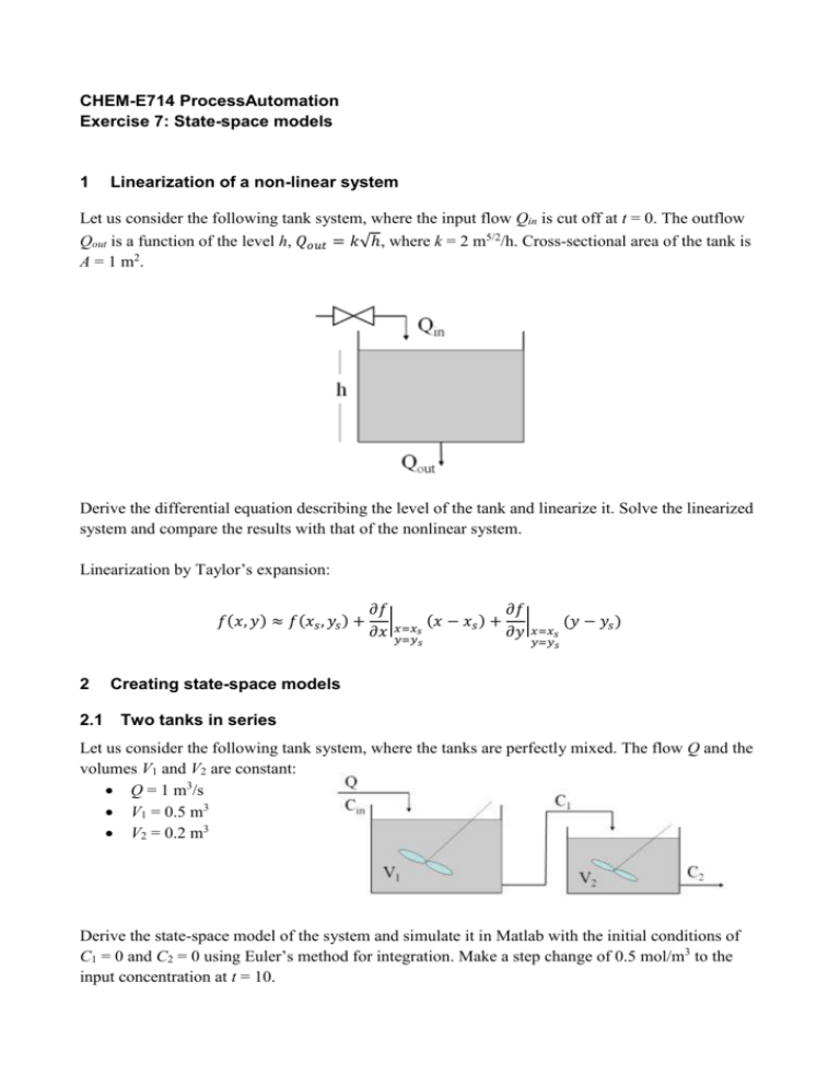
CHEM-E714 ProcessAutomation
Exercise 7: State-space models
1
Linearization of a non-linear system
Let us consider the following tank system, where the input flow Qin is cut off at t = 0. The outflow
Qout is a function of the level h, 𝑄𝑜𝑢𝑡 = 𝑘√ℎ, where k = 2 m5/2/h. Cross-sectional area of the tank is
A = 1 m2 .
Derive the differential equation describing the level of the tank and linearize it. Solve the linearized
system and compare the results with that of the nonlinear system.
Linearization by Taylor’s expansion:
𝑓(𝑥, 𝑦) ≈ 𝑓(𝑥𝑠 , 𝑦𝑠 ) +
𝜕𝑓
𝜕𝑓
|𝑥=𝑥 (𝑥 − 𝑥𝑠 ) + |
(𝑦 − 𝑦𝑠 )
𝜕𝑥 𝑦=𝑦𝑠
𝜕𝑦 𝑥=𝑥𝑠
𝑠
2
2.1
𝑦=𝑦𝑠
Creating state-space models
Two tanks in series
Let us consider the following tank system, where the tanks are perfectly mixed. The flow Q and the
volumes V1 and V2 are constant:
 Q = 1 m3/s
 V1 = 0.5 m3
 V2 = 0.2 m3
Derive the state-space model of the system and simulate it in Matlab with the initial conditions of
C1 = 0 and C2 = 0 using Euler’s method for integration. Make a step change of 0.5 mol/m3 to the
input concentration at t = 10.
2.2
Isothermal reactor
Consider the following reaction scheme, taking place in an isothermal reactor:
k1
k2
A 
B 
C
k3
2 A 
D
with the following molar rates of formation:
 k1 = 5/6 min-1
 k2 = 5/3 min-1
 k3 = 1/6 l/mol min
Assuming that the feed stream contains only component A, with initial concentration CA0 = 10,
define the state-space model and study the formation of B in the following cases:
 The dilution rate is Fs/V = 4/7 min-1;
 The dilution rate is Fs/V = 2,8744 min-1;
This reaction scheme was presented by Van de Vusse (1964) and it turned out that this type of
system can have significantly different input/output characteristics, depending on the chosen
operating condition.
Solutions
1 Linearization
Before linearizing the previous function, we need to find the steady-state operating point. That is
dh
obtained by solving the dynamic equation for
= 0, in order to get hss. Using a truncated Taylor
dt
series expansion, we find:
Q
 1
k
k
h  hss 
f (h, Qin )   in,ss 
hss   Qin  Qin, ss  
A
2 A hss
 A
 A
The first term on the right hand side is zero, because the linearization is about a steady-state point.
That is:
Qin,ss k
dh

hss  0
hss ,Qin , ss 
dt
A
A
We can now write:
d (h  hss ) 1
k
h  hss 
 Qin  Qin, ss  
dt
A
2 A hss
and using deviation notation (h’ = h - hss and Q’ = Q - Qss), and dropping the ≈
dh ' 1 '
k
 Q in 
h'
dt A
2 A hss
Taking the Laplace transform, we get:
1
k
s H ( s)  Qin ( s) 
H ( s)
A
2 A hss
and then, the transfer function:
1
H ( s)
A

k
Qin ( s )
s
2 A hss
Using the numerical values, we get:
G (s) 
1
s 1
There is a step-like change in Q in' = -2m3/h, that in Laplace domain is Qin(s) = -21/s . Follows:
H ( s)  G ( s) Qin ( s)
H ( s)  
1 2
s 1 s
Taking the inverse transform, we get the dynamic behavior:
L
-1
H (s) 
L
-1 
2 
 s ( s  1)   h ' (t )


From the table, we get:
h’(t) = -2(1 – e-t)
Finally,
h(t) = hss + h’(t) = 2et - 1
(1)
Differential equation
Solving the differential equation:
dh 1
 (Qin  k h )
dt
A
with an initial value h(0) = 1m and Qin = 0 m3/h, h = 2 m5/2/h, A = 1m, we get:
dh
 2 h
dt
and integrating:
h(t )  (1  t ) 2
(2)
To compare the different results, we plot the curves in Equation (1) and (2), in Figure 2.2.
2.1 Two tanks in series
In order to define the system of differential equations for the given system, we consider the mass
balance equations around the two reactors and we get:
dC
V1 1  Q(C in  C1 )
dt
dC 2
V2
 Q(C1  C 2 )
dt
Substituting the numerical values, we have:
dC1
 2C in  2C1
dt
dC 2
 5C1  5C 2
dt
That can be written as a state space model:
 
0 C1  2
C1    2

C

    5  5  C 2  0  in
C 2 
which has the general form:

x = Ax + Bu
where
  2 0
A= 

 5  5
2
B=  
0 
The state and the input vectors are (notice that the input is a scalar):
x 
x =  1  and
u = C in
 x2 
It should be noticed that for linear systems, we can write the deviation variable model directly from
the physical model, skipping the intermediate steps. The additional equation that is normally
associated with a state model is
y = Cx + Du
where
y is the vector of output variables
Generally, output variables are variables that can be measured (at least conceptually) or are of
particular interest in a simulation study. Here, we consider the output from the second reactor as the
only output for our system and we get:
y = 0 1 x
To define the transfer function for the system, we need to take first the Laplace transform
of the system:
sC1(s) = -2C1(s) + 2Cin(s)
sC2(s) = 5C1(s) - 5C2(s)
That can be also written as:
sX(s) = AX(s) + BU(s)
Y (s) = CX(s)
Now, we can act in two ways:
Calculating the transfer function directly from the system equations:
G ( s)
G( s)  2
Gin (s)
we get:
G( s) 
10
( s  2)( s  5)
Calculating the transfer function using matrices:
Y (s)
G (s) 
 C (sI - A)-1 B
U (s)
s  2
G( s)  0 1 
 5
0 
s  5
1
 2
0
 
we get:
G( s) 
10
( s  2)( s  5)
The weighting function is the inverse transform of the function G(s) (from the table):
1
1
G( s) 
 g (t ) 
(e bt  e at )
( s  a)( s  b)
a b
that is:
10
10
G( s) 
 g (t )  (e 2t  e 5t )
( s  2)( s  5)
3
The step input is the most common input forcing function; it is used to solve dynamic problems
where a sudden change in the input variable occurs. In the Laplace domain, if A is the step
amplitude, we have:
A
L 
s
Considering a unit step, we get:
1
Y (s)  G(s)
s
10
1
Y (s) 
( s  2)( s  5) s
The step response is the inverse of the function Y (s):
t
1
0 f (t )  s Ff (t )  F (s)
5
2
y (t )  1  e  2t  e 5t
3
3
Matlab
The transfer function using Matlab can be easily found, with the routine ss2tf that can be used to
convert a state-space model to a transfer function model. After entering the matrices A, B, C and D,
the command:
[num,den] = ss2tf(A,B,C,D,iu)
will generate the numerator and denominator Laplace domain polynomials from the transfer
function between input number iu and the outputs.
The Matlab step function assumes a deviation variable form (the initial conditions are zero). The
command is:
step(SYS)
which plots the step response of the LTI model SYS
2.2 Isothermal reactor
Assuming constant density and constant volume, we first note that the overall mass balance simply
gives F = F0.
Component A Balance
dC A
F
 (C A0  C A )  k1C A  k 3C A2
dt
V
(3)
Component B Balance
dC B
F
(4)
  C B  k1C A  k 2 C B
dt
V
Component C Balance
dCC
F
(5)
  CC  k 2 C B
dt
V
Component D Balance
dC D
F
1
(6)
  C D  k 3C A2
dt
V
2
Since we are interested in the production of the component B and since Equations (3) and (4) do not
depend on CC and CD, we need to solve only those Equations.
Steady-State
Solving for the steady-state for Equation (3), we find a quadratic equation in CA and solving it
(using only the positive root):
C As 
F
F
F
1
(  ( k1  s )  ( k1  s ) 2  4 k 3 s C A 0 )
2k 3
V
V
V
and solving for CB:
C Bs 
k1C As
Fs
 k2
V
State-Space Model
We linearize the nonlinear modeling equations to find the state space form, where the state, input
and output vector are, deviation form:
C  C As 
C  C As 
F F 
x=  A
,
u =   s ,
y=  A


V V 
C B  C Bs 
C B  C Bs 
The elements of the state-space A are found as Aij  f i x j , where f1 is the balance of x1 = CA and
f2 is the balance of x2 = CB:
a11 
F
f1
  s  k1  2k 3C As
x1
V
b11 
f1
 C A0 s  C As
u1
a12 
f1
0
x 2
b21 
f 2
 C Bs
u1
a 21 
f 2
 k1
x1
a 22 
F
f 2
  s  k2
x 2
V
The state-space model is:
 Fs

 k1  2k 3C As
A =  V

k1


 , B = C A0 s  C As 
 C


Fs
Bs




 k2

V

0
Case 1
Considering a dilution rate of Fs/V = 4/7 min-1, we obtain the following steady-state concentration:
CAs = 3 mol/liter
CBs = 1,117 mol/liter
which yield to:
A =  2,4048
0
,B=

 0,8333  2,2381
 7,0000
 1,1170 


The process transfer function relating input 1 and output 2 is:
G ( s) 
 1,117 s  3,1472
s  4,6429s  5,3821
2
Case 2
Considering a dilution rate of Fs/V = 2,8744 min-1, we obtain the following steady-state
concentration:
CAs = 6,0870 mol/liter
CBs = 1,117 mol/liter
which yield to:
A =  5,7367
0
 , B =  3,9130 

 1,1170 
 0,8333  4,5411


The process transfer function relating input 1 and output 2 is:
G ( s) 
 1,117 s  3,1472
s  10,2778  26,0508
2