Correlation and Regression Analysis: SPSS
Bivariate Analysis: Cyberloafing Predicted from Personality and Age
These days many employees, during work hours, spend time on the Internet doing personal
things, things not related to their work. This is called “cyberloafing.” Research at ECU, by Mike
Sage, graduate student in Industrial/Organizational Psychology, has related the frequency of
cyberloafing to personality and age. Personality was measured with a Big Five instrument.
Cyberloafing was measured with an instrument designed for this research. Age is in years. The
cyberloafing instrument consisted of 23 questions about cyberloafing behaviors, such as “shop online
for personal goods,” “send non-work-related e-mail,” and “use Facebook.” For each item,
respondents were asked how often they engage in the specified activity during work hours for
personal reasons. The response options were “Never,” “Rarely (about once a month),” “Sometimes
(at least once a week),” and “Frequently (at least once a day).” Higher scores indicate greater
frequency of cyberloafing.
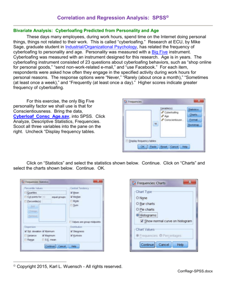
For this exercise, the only Big Five
personality factor we shall use is that for
Conscientiousness. Bring the data,
Cyberloaf_Consc_Age.sav, into SPSS. Click
Analyze, Descriptive Statistics, Frequencies.
Scoot all three variables into the pane on the
right. Uncheck “Display frequency tables.
Click on “Statistics” and select the statistics shown below. Continue. Click on “Charts” and
select the charts shown below. Continue. OK.

Copyright 2015, Karl L. Wuensch - All rights reserved.
CorrRegr-SPSS.docx
2
The output will show that age is positively skewed, but not quite badly enough to require us to
transform it to pull in that upper tail. Click Analyze, Correlate, Bivariate. Move all three variables into
the Variables box. Ask for Pearson and Spearman coefficients, two-tailed, flagging significant
coefficients. Click OK. Look at the output. With both Pearson and Spearman, the correlations
between cyberloafing and both age and Conscientiousness are negative, significant, and of
considerable magnitude. The correlation between age and Conscientiousness is small and not
significant.
Click Analyze, Regression, Linear. Scoot the Cyberloafing variable into the Dependent box
and Conscientiousness into the Independent(s) box.
3
Click Statistics. Select the statistics shown below. Continue. Click Plots. Select the plot
shown below. Continue, OK.
Look at the output. You get the same value of r obtained with the correlation analysis, of
course. The r2 shows that our linear model explains 32% of the variance in cyberloafing. The
adjusted R2, also known as the “shrunken R2,” is a relatively unbiased estimator of the population 2.
For a bivariate regression it is computed as:
2
rshrunken
 1
(1  r 2 )( n  1)
.
(n  2)
The residuals statistics show that there no cases with a standardized residual beyond three
standard deviations from zero. If there were, they would be cases where the predicted value was
very far from the actual value and we would want to investigate such cases. The histogram shows
that the residuals are approximately normally distributed, which is assumed when we use t or F to get
a p value or a confidence interval.
Let’s now create a scatterplot. Click Graphs, Legacy Dialogs, Scatter/Dot, Simple Scatter,
Define. Scoot Cyberloafing into the Y axis box and Conscientiousness into the X axis box. Click OK.
4
Go to the Output window and double click on the chart to open the chart editor. Click
Elements, Fit Line at Total, Fit Method = Linear, Close.
You can also ask SPSS to
draw confidence bands on the plot,
for predicting the mean Y given X, or
individual Y given X, or both (to get
both, you have to apply the one,
close the editor, open the editor
again, apply the other).
5
You can also edit the shape, density, and color of the markers and the lines. While in the
Chart Editor, you can Edit, Copy Chart and then paste the chart into Word. You can even ask SPSS
to put in a quadratic (Y = a +b1X + b2X2 + error) or cubic (Y = a +b1X + b2X2 +b3X3 + error) regression
line.
Construct a Confidence Interval for . Try the calculator at Vassar. Enter the value of r and
sample size and click “Calculate.”
Presenting the Results of a Correlation/Regression Analysis. Employees’ frequency of
cyberloafing (CL) was found to be significantly, negatively correlated with their Conscientiousness
(CO), r(N = 51) = -.563, p < .001, 95% CI [-.725, -.341], CL = 57.04 - .864(CO).
Trivariate Analysis: Age as a Second Predictor
Click Analyze, Regression, Linear. Scoot the Cyberloafing variable into the Dependent box
and both Conscientiousness and Age into the Independents box. Click Statistics and check Part and
Partial Correlations, Casewise Diagnostics, and Collinearity Diagnostics (Estimates and Model Fit
should already be checked). Click Continue. Click Plots. Scoot *ZRESID into the Y box and
*ZPRED into the X box. Check the Histogram box and then click Continue. Click Continue, OK.
When you look at the output for this multiple regression, you see that the two predictor model
does do significantly better than chance at predicting cyberloafing, F(2, 48) = 20.91, p < .001. The F
in the ANOVA table tests the null hypothesis that the multiple correlation coefficient, R, is zero in the
population. If that null hypothesis were true, then using the regression equation would be no better
6
than just using the mean for cyberloafing as the predicted cyberloafing score for every person.
Clearly we can predict cyberloafing significantly better with the regression equation rather than
without it, but do we really need the age variable in the model? Is this model significantly better than
the model that had only Conscientiousness as a predictor? To answer that question, we need to look
at the "Coefficients," which give us measures of the partial effect of each predictor, above and beyond
the effect of the other predictor(s).
The Regression Coefficients
The regression equation gives us two unstandardized slopes, both of which are partial
statistics. The amount by which cyberloafing changes for each one point increase in
Conscientiousness, above and beyond any change associated with age, is -.779, and the amount by
which cyberloafing changes for each one point increase in age, above and beyond any change
associated with Conscientiousness, is -.276. The intercept, 64.07, is just a reference point, the
predicted cyberloafing score for a person whose Conscientiousness and age are both zero (which are
not even possible values). The "Standardized Coefficients" (usually called beta,  ) are the slopes in
standardized units -- that is, how many standard deviations does cyberloafing change for each one
standard deviation increase in the predictor, above and beyond the effect of the other predictor(s).
The regression equation represents a plane in three dimensional space (the three dimensions
being cyberloafing, Conscientiousness, and age). If we plotted our data in three dimensional space,
that plane would minimize the sum of squared deviations between the data and the plane. If we had
a 3rd predictor variable, then we would have four dimensions, each perpendicular to each other
dimension, and we would be out in hyperspace.
Tests of Significance
The t testing the null hypothesis that the intercept is zero is of no interest, but those testing the
partial slopes are. Conscientiousness does make a significant, unique, contribution towards
predicting AR, t(48) = 4.759, p < .001. Likewise, age also makes a significant, unique, contribution,
t(48) = 3.653, p = .001 Please note that the values for the partial coefficients that you get in a
multiple regression are highly dependent on the context provided by the other variables in a model. If
you get a small partial coefficient, that could mean that the predictor is not well associated with the
dependent variable, or it could be due to the predictor just being highly redundant with one or more of
the other variables in the model. Imagine that we were foolish enough to include, as a third predictor
in our model, students’ score on the Conscientiousness and age variables added together. Assume
that we made just a few minor errors when computing this sum. In this case, each of the predictors
would be highly redundant with the other predictors, and all would have partial coefficients close to
zero. Why did I specify that we made a few minor errors when computing the sum? Well, if we didn’t,
then there would be total redundancy (at least one of the predictor variables being a perfect linear
combination of the other predictor variables), which causes the intercorrelation matrix among the
predictors to be singular. Singular intercorrelation matrices cannot be inverted, and inversion of that
matrix is necessary to complete the multiple regression analysis. In other words, the computer
program would just crash. When predictor variables are highly (but not perfectly) correlated with one
another, the program may warn you of multicollinearity. This problem is associated with a lack of
stability of the regression coefficients. In this case, were you randomly to obtain another sample from
the same population and repeat the analysis, there is a very good chance that the results (the
estimated regression coefficients) would be very different.
Multicollinearity
Multicollinearity is a problem when for any predictor the R2 between that predictor and the
remaining predictors is very high. Upon request, SPSS will give you two transformations of the
squared multiple correlation coefficients. One is tolerance, which is simply 1 minus that R2. The
second is VIF, the variance inflation factor, which is simply the reciprocal of the tolerance. Very low
7
values of tolerance (.1 or less) indicate a problem. Very high values of VIF (10 or more, although
some would say 5 or even 4) indicate a problem. As you can see in the table below, we have no
multicollinearity problem here.
Coefficientsa
Model
Collinearity Statistics
Tolerance
1
VIF
Age
.980
1.021
Conscientiousness
.980
1.021
Partial and Semipartial Correlation Coefficients
I am going to use a Venn diagram to help explain what squared partial and semipartial
correlation coefficients are.. Look at the ballantine below.
The top circle represents variance in cyberloafing, the right circle that in age, the left circle that in
Conscientiousness. The overlap between circle Age and Cyberloaf, area A + B, represents the r2
between cyberloafing and age. Area B + C represents the r2 between cyberloafing and
Conscientiousness. Area A + B + C + D represents all the variance in cyberloafing, and we
standardize it to 1. Area A + B + C represents the variance in cyberloafing explained by our best
weighted linear combination of age and Conscientiousness, 46.6% (R2). The proportion of all of the
variance in cyberloafing which is explained by age but not by Conscientiousness is equal to:
A
A
  A.
A B C  D 1
Area A represents the squared semipartial correlation for age (.149). Area C represents the
squared semipartial correlation for Conscientiousness (.252). SPSS gives you the unsquared
semipartial correlation coefficients, but calls them "part correlations."
Although I generally prefer semipartial correlation coefficients, some persons report the partial
correlation coefficients, which are provided by SPSS. The partial correlation coefficient will always
be at least as large as the semipartial, and almost always larger. To treat it as a proportion, we
obtain the squared partial correlation coefficient. In our Venn diagram, the squared partial
C
correlation coefficient for Conscientiousness is represented by the proportion
. That is, of the
CD
variance in cyberloafing that is not explained by age, what proportion is explained by
Conscientiousness? Or, put another way, if we already had age in our prediction model, by what
proportion could we reduce the error variance if we added Conscientiousness to the model? If you
consider that (C + D) is between 0 and 1, you should understand why the partial coefficient will be
larger than the semipartial.
8
If we take age back out of the model, the r2 drops to .317. That drop, .466 - .317 = .149, is
the squared semipartial correlation coefficient for age. In other words, we can think of the squared
semipartial correlation coefficient as the amount by which the R2 drops if we delete a predictor from
the model.
If we refer back to our Venn diagram, the R2 is represented by the area A+B+C, and the
redundancy between misanthropy and idealism by area B. The redundant area is counted (once) in
the multiple R2, but not in the partial statistics.
Checking the Residuals
For each subject, the residual is the subject’s actual Y score minus the Y score as predicted
from the regression solution. When we use t or F to test hypotheses about regression parameters or
to construct confidence intervals, we assume that, in the population, those residuals are normally
distributed and constant in variance.
The histogram shows the marginal distribution of the residuals. We have assumed that this is
normal.
The plot of the standardized residuals (standardized difference between actual cyberloafing
score and that predicted from the model) versus standardized predicted values allows you to evaluate
the normality and homescedasticity assumptions made when testing the significance of the model
and its parameters. Open the chart in the editor and click Options, Y-axis reference line to draw a
horizontal line at residual = 0. If the normality assumption has been met, then a vertical column of
residuals at any point on that line will be normally distributed. In that case, the density of the plotted
symbols will be greatest near that line, and drop quickly away from the line, and will be symmetrically
distributed on the two sides (upper versus lower) of the line. If the homoscedasticity assumption
has been met, then the spread of the dots, in the vertical dimension, will be the same at any one point
on that line as it is at any other point on that line. Thus, a residuals plot can be used, by the trained
eye, to detect violations of the assumptions of the regression analysis. The trained eye can also
detect, from the residual plot, patterns that suggest that the relationship between predictor and
criterion is not linear, but rather curvilinear.
Residuals can also be used to identify any cases with large residuals – that is, cases where
the actual Y differs greatly from the predicted Y. Such cases are suspicious and should be
investigated. They may represent for which the data were incorrectly entered into the data file or for
9
which there was some problem during data collection. They may represent cases that are not
properly considered part of the population to which we wish to generalize our results. One should
investigate cases where the standardized residual has an absolute value greater than 3 (some would
say 2).
Importance of Looking at a Scatterplot Before You Analyze Your Data
It is very important to look at a plot of your data prior to conducting a linear
correlation/regression analysis. Close the Cyberloaf_Consc_Age.sav file and bring Corr_Regr.sav
into SPSS. From the Data Editor, click Data, Split File, Compare Groups, and scoot Set into the
"Organize output by groups" box. Click OK.
Next, click Analyze, Regression, Linear. Scoot Y into the Dependent box and X into the
Independent(s) box. Click Stat and ask for Descriptives (Estimates and Model Fit should already be
selected). Click Continue, OK.
Next, click Graphs, Scatter, Simple. Identify Y as the Y variable and X as the X variable. Click
OK.
Look at the output. For each of the data sets, the mean on X is 9, the mean on Y is 7.5, the
standard deviation for X is 3.32, the standard deviation for Y is 2.03, the r is .816, and the regression
equation is Y = 3 + .5X – but now look at the plots. In Set A, we have a plot that looks about like what
we would expect for a moderate to large positive correlation. In set B we see that the relationship is
really curvilinear, and that the data could be fit much better with a curved line (a polynomial function,
quadratic, would fit them well). In Set C we see that, with the exception of one outlier, the relationship
is nearly perfect linear. In set D we see that the relationship would be zero if we eliminated the one
extreme outlier -- with no variance in X, there can be no covariance with Y.
Moderation Analysis
Sometimes a third variable moderates (alters) the relationship between two (or more) variables
of interest. You are about to learn how to conduct a simple moderation analysis.
One day as I sat in the living room, watching the news on TV, there was a story about some
demonstration by animal rights activists. I found myself agreeing with them to a greater extent than I
normally do. While pondering why I found their position more appealing than usual that evening, I
noted that I was also in a rather misanthropic mood that day. That suggested to me that there might
be an association between misanthropy and support for animal rights. When evaluating the ethical
status of an action that does some harm to a nonhuman animal, I generally do a cost/benefit analysis,
weighing the benefit to humankind against the cost of harm done to the nonhuman. When doing such
an analysis, if one does not think much of humankind (is misanthropic), e is unlikely to be able to
justify harming nonhumans. To the extent that one does not like humans, one will not be likely to
10
think that benefits to humans can justify doing harm to nonhumans. I decided to investigate the
relationship between misanthropy and support of animal rights.
Mike Poteat and I developed an animal rights questionnaire, and I developed a few questions
designed to measure misanthropy. One of our graduate students, Kevin Jenkins, collected the data
we shall analyze here. His respondents were students at ECU. I used reliability and factor analysis
to evaluate the scales (I threw a few items out). All of the items were Likert-type items, on a 5-point
scale. For each scale, we computed each respondent's mean on the items included in that scale.
The scale ran from 1 (strongly disagree) to 5 (strongly agree). On the Animal Rights scale (AR), high
scores represent support of animal rights positions (such as not eating meat, not wearing leather, not
doing research on animals, etc.). On the Misanthropy scale (MISANTH), high scores represent high
misanthropy (such as agreeing with the statement that humans are basically wicked).
The idealist is one who believes that morally correct behavior always leads only to desirable
consequences; an action that leads to any bad consequences is a morally wrong action. Thus, one
would expect the idealist not to engage in cost/benefit analysis of the morality of an action -- any bad
consequences cannot be cancelled out by associated good consequences. Thus, there should not
be any relationship between misanthropy and attitude about animals in idealists, but there should be
such a relationship in nonidealists (who do engage in such cost/benefit analysis, and who may, if they
are misanthropic, discount the benefit to humans).
Accordingly, a proper test of my hypothesis would be one that compared the relationship
between misanthropy and attitude about animals for idealists versus for nonidealists. Although I did a
more sophisticated analysis than is presented here (a "Potthoff analysis," which I cover in my
advanced courses), the analysis presented here does address the question I posed. Based on a
scores on the measure of idealism, each participant was classified as being either an idealist or not
an idealist. Now all we need to do is look at the relationship between misanthropy and idealism
separately for idealists and for nonidealists.
Bring into SPSS the data file Poffhoff.sav. From the Data Editor, click Data, Split File,
Organize Output by Groups. Scoot the Idealism variable into the "Groups based on" box. Click OK.
Click Analyze, Regression, Linear. Scoot AR into the Dependent box, Misanth into the
Independent(s) box. Click Statistics. Check Descriptives (Estimates and Model Fit should already be
checked). Click Continue, OK.
Make some scatter plots too, with the regression line drawn in. Click Graphs, Legacy
Dialogues, Scatter/Dot, Simple Scatter, Define. Scoot AR into the Y axis box and Misanth into the X
axis box. Click OK. Go to the Output window and double click on each chart to open the chart editor.
Click Elements, Fit Line at Total, Fit Method = Linear, Close.
The output for the nonidealists shows that the relationship between attitude about animals and
misanthropy is significant ( p < .001) and of nontrivial magnitude ( r = .364, n = 91). The plot shows a
nice positive slope for the regression line. With nonidealists, misanthropy does produce a discounting
of the value of using animals for human benefit, and, accordingly, stronger support for animal rights.
On the other hand, with the idealists, who do not do cost/benefit analysis, there is absolutely no
relationship between misanthropy and attitude towards animals. The correlation is trivial ( r = .020, n
= 63) and nonsignificant ( p = .87), and the plot shows the regression line to be flat.
You can find a paper based on these data at:
http://core.ecu.edu/psyc/wuenschk/Animals/ABS99-ppr.htm
11
Group Differences in Unstandardized Slopes and in Correlation Coefficients
Please remember that the relationship between X and Y could differ with respect to the slope
for predicting Y from X, but not with respect to the Pearson r, or vice versa The Pearson r really
measures how little scatter there is around the regression line (error in prediction), not how steep the
regression line is.
On the left, we can see that the slope is the same for the relationship plotted with blue o’s and
that plotted with red x’s, but there is more error in prediction (a smaller Pearson r ) with the blue o’s.
For the blue data, the effect of extraneous variables on the predicted variable is greater than it is with
the red data.
On the right, we can see that the slope is clearly higher with the red x’s than with the blue o’s,
but the Pearson r is about the same for both sets of data. We can predict equally well in both groups,
but the Y variable increases much more rapidly with the X variable in the red group than in the blue.
Placing a Confidence Interval on Multiple R or R2
Please see my document Putting Confidence Intervals on R2 or R.
Presenting the Results of a Multiple Linear Correlation/Regression Analysis
Please read the article at http://jolt.merlot.org/vol5no2/wuensch_0609.pdf and pay special
attention to how the results of the multiple regression analyses were presented, including Tables 3
and 4. This is the style I would expect you to use when presenting the results of a multiple regression
were such an analysis to be on the an assignment or examination.
Annotated Output for This Lesson
Return to my SPSS Lessons page
More Lessons on Multiple Regression
Multiple Regression With SAS
Producing and Interpreting Residuals Plots in SPSS
Copyright 2015, Karl L. Wuensch - All rights reserved.