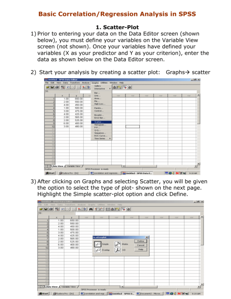
Basic Correlation/Regression Analysis in SPSS
1. Scatter-Plot
1) Prior to entering your data on the Data Editor screen (shown
below), you must define your variables on the Variable View
screen (not shown). Once your variables have defined your
variables (X as your predictor and Y as your criterion), enter the
data as shown below on the Data Editor screen.
2) Start your analysis by creating a scatter plot:
Graphs scatter
3) After clicking on Graphs and selecting Scatter, you will be given
the option to select the type of plot- shown on the next page.
Highlight the Simple scatter-plot option and click Define.
4) After the Simple Scatter-plot window appears, move your
criterion variable into the Y axis slot and your predictor variable
into the X axis slot (shown below). Click on OK.
5) The scatter plot will be produced and displayed on the Output
Viewer.
2. Regression Analysis
After creating a scatter plot, you should run a regression analysis.
The regression analysis will produce regression coefficients, a
correlation coefficient, and an ANOVA table.
1) Begin by selecting AnalyzeRegression Linear (shown below).
2) Once the Linear Regression window appears (shown below), move
your criterion variable into the Dependent slot and your predictor
variable into the Independent slot. Click OK.
3) The output of the analysis is shown below. The Model Summary
table reports the correlation coefficient as R (note it should be a
lower case r for bivariate correlation, but it isn’t). The R Square
statistic is in the second column and is also known as “proportionate
reduction in error”or “variance accounted for.”
The second table is the ANOVA summary table that tests the null
hypothesis. In the case of correlation the null hypothesis is that the
correlation is zero. In this case we reject the null hypothesis because
the p value is less than .05. In this case the p value is .003.
The final table presents the regression coefficients. Looking at the
Un-standardized Coefficients column you see B weights. The B weight
(613.611) in the Constant row is referred to as the intercept. The B
weight (-39.861) in the predictor row (Birth Order) is referred to as
the slope. Note that the correlation will be negative when the slope
has a negative value. These coefficients are used to form the
following linear regression equation.
y =613.61 - 39.86x