Modeling and simulation methods in nanotechnology.
Practical laboratory
Solving practical tasks in computer laboratory. 6 hours/topic
Practical application of tight-binding method to numerical
calculations of energy bands in selected graphene structures.
Task 1.
One-dimensional chain of atoms. Construction of molecular orbital and Hamiltonian
matrix.
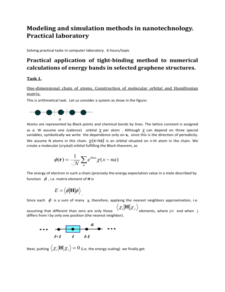
This is arithmetical task. Let us consider a system as show in the figure:
Atoms are represented by Black points and chemical bonds by lines. The lattice constant is assigned
as a. W assume one (valence) orbital per atom . Although can depend on three special
variables, symbolically we write the dependence only on x, since this is the direction of periodicity.
We assume N atoms in this chain. x-na) is an orbital situated on n-th atom in the chain. We
create a molecular (crystal) orbital fulfilling the Bloch theorem, as
 (r ) 
1
N
e
ikna
 ( x  na)
n
The energy of electron in such a chain (precisely the energy expectation value in a state described by
function

, i.e. matrix element of H is
E   H
Since each

.
is a sum of many χ, therefore, applying the nearest neighbors approximation, i.e.
i H  j
assuming that different than zero are only those
differs from I by only one position (the nearest neighbor).
Next, putting
 i H  i  0 (i.e. the energy scaling)
elements, where j=i and when j
we finally get
E   0 H 1 e ikd   0 H  1 e ikd  t 2 cos( kd )
(1)
that means a single band E(k).
Students have to derive the formula (1) and draw E(k) in any graphical tool.
Task 2.
One-dimensional chain as in task.1, but now unit cell contains two atoms.
The aims of this exercise are: (1) derive formula for Hamiltonian matrix elements, (2)
understanding that the resulting bands, come out are energetically equivalent to the band obtained
in task.1, (3) to show that the bands can be obtained by folding BZ from the task.1. Now, we have
the same chain but the unit cell is defined in a different way.
Now, the dimension of Hamiltonian matrix is 2 (two atoms in a unit cell). Setting diagonal elements
equal zero we get

0
t (1  eikd )
H 

ikd
t
(
1

e
)
0


The energy spectrum is the same as in task.1, although now built of two bands. It is important to
notice the difference in the size of BZ in both cases. Matrix can be diagonalized “by hand” or one can
write a code , which will construct H and call appropriate procedure (diagonalization).
Task 3.
Construction of the Hamiltonian matrix for a few-atomic molecule.
For ex ample, „molecule” C4
Hii = 0 , i=1,2,3,4 - as diagonal elements, H12 = H21 = H23 = H32 = H34 = H43 = t [ = -2.7 eV ] All the others
Hkl = 0; here H doesn’t depend on k
Task4.
Construction of the Hamiltonian matrix for the simplest (the most narrow) armchair
graphene Ribbon.
First, one has to enumerate all the nodes (atoms) in t hunt cell (also separately in the neighbor unit
cells).
 0

t
H 
 0
 ikd
t (e )
t 0 t (e ikd )

0 t
0 
t 0
t 

0 t
0 
Task 5.
Construction of the Hamiltonian matrix for the simplest (the most narrow) zigzag
graphene Ribbon.
First, one has to enumerate all the nodes (atoms) in t hunt cell (also separately in the neighbor unit
cells).


0
t (1  eikd )
0
0


t (1  e ikd )
0
t
0


H
ikd 

0
t
0
t (1  e )


ikd
0
0
t (1  e )
0


Task 6.
Construction of the Hamiltonian matrix for carbon nanotube (3,3)
And matrix H (dimension = 12)

0
t (1  e ikd )
0
0
0
0
0
0
0

 ikd
0
t
0
0
0
0
0
0
t (1  e )
 ikd

0
t
0
t (1  e )
0
0
0
0
0

ikd
0
0
t (1  e )
0
t
0
0
0
0

ikd

0
0
0
t
0
t (1  e )
0
0
0

 ikd
0
0
0
0
t (1  e )
0
t
0
0


0
0
0
0
0
t
0
t (1  e ikd )
0

ikd

0
0
0
0
0
0
t (1  e )
0
t

0
0
0
0
0
0
0
t


etc...




0
0
0
0
0
0
0
0
0
0
0
0
0
0
0
0
t

0
0

0
0

0
0

0







Final classification task.
Construction and execution of a computer code for calculating energy structure of any
graphene systems, periodic and non-periodic ones.
General structure of the code:
 Determination of the number of nodes atoms) in the unit cell, N= dimH,
 Definition of bonds (connections) within a given unit cell; determination of elements, which
are Hij = t,
 Definition of connections (bonds) between atoms belonging to neighbor unit cells, (te(ik), or
t[1+eik]),
 Loop over all k values (in BZ)
- diagonalization of H for each k, using any appropriate method, depending on the
programming language or package and platform chosen,
 Allow for different strengths of Bond (t) in different regions,
 Allow for unit cell modification by adding or removing atoms,
 Write the results (energy bands) down to a file
 Make diagrams of the calculated energy bands.
Students can chose any language or computational package they wish Fortran, C, C++, Csharp,
Matlab, Phyton, etc..). They can utilize ready-to-use libraries and procedures for diagonalization of
complex, hermitian matrices.
For classification, students must demonstrate they now their codes in detail. They must execute
the code for a system chosen by the teacher (e.g., carbon tube (6,6), carbon tube (5,0), graphene
zigzag Ribbon with one edge modified by different number of Klein nodes).
Resonance states in nanostructures
Three exercise problems (Tasks 7-9) associated with resonances in nanostructures are given here.
They should be done by single students within the exercise hours in a computer laboratory or at
home. One of them should be chosen by the teacher for a group of students or for a given course. (A
student is expected to do one of the exercises). The job is to prepare some analytical formulas, to
encode them, to compute the results and to present them graphically. Students choose which
programming language and what programming environments they want to use.
Task 7.
Resonance states of symmetric system of one well and two barriers
The system consists of three layers of semiconductors. We consider one electron whose interaction
with the structure is modeled by a one-dimensional potential of rectangular well and barriers:
0,
𝑉𝑜 ,
𝑉(𝑥) = 0,
𝑉𝑜 ,
{ 0,
𝑥 < −𝑏
−𝑏 ≤ 𝑥 ≤ −𝑎
|𝑥| < 𝑎
𝑎≤𝑥≤𝑏
𝑥≥𝑏
where 𝑉𝑜 > 0.
The Hamiltonian is:
̂=−
𝐻
1 𝑑2
+ 𝑉(𝑥).
2𝑚 𝑑𝑥 2
We have to solve the Schroedinger equation for energies of the range between 0 and 𝑉𝑜 in a way
analogous to that described in the lecture chapter “Resonance states of the potential well-barrier
system”. The symmetry of the system should be used to simplify the problem. Since the system does
not change under inversion of coordinate 𝑥 → −𝑥, i.e. , 𝑉(−𝑥) = 𝑉(𝑥), the probability distribution
also has to be even function of 𝑥 , i.e. |𝜓(−𝑥)|2 = |𝜓(𝑥)|2 . Functions themselves can be either
even, 𝜓(−𝑥) = 𝜓(𝑥), or odd, 𝜓(−𝑥) = − 𝜓(𝑥). Eigenfunctions of these two types can be found
separately. Thus we assume proper relations between coefficient present in the functions on the left
and right sides. This reduces the number of unknowns and makes the problem easier.
The results should be presented in a graphical way. Especially the resonance character of solutions
should be shown like in the lecture chapter “Resonance states of the potential well-barrier system”.
New ideas on how to present results are welcome.
The computer code should offer possibility of changing the parameters of the potential 𝑎, 𝑏, 𝑉𝑜 and
effective mass of the electron 𝑚.
Task 8.
Resonance states of a symmetric nanolayer-structure modeled with an analytical
potential
The nanostructure under consideration is similar to that of previous exercise but modeled with an
analytical (continuous) potential
2
𝑉(𝑥) = (𝑎𝑥 2 − 𝑏)𝑒 −𝑞𝑥 ,
where 𝑎, 𝑏 i 𝑞 are nonnegative real parameters.
The Hamiltonian is
̂=−
𝐻
1 𝑑2
+ 𝑉(𝑥).
2𝑚 𝑑𝑥 2
The exercise relies in application of the stabilization method to find resonance states in the energy
range from the potential asymptote (energy level equal to lim 𝑉(𝑥) = 0 ) up to the maximum of
𝑥→∞
the potential and bound states of energies between the minimum of the potential (– 𝑏) and the
asymptote.
The symmetry of the system( 𝑉(−𝑥) = 𝑉(𝑥)) should be used; the even and odd solutions should be
searched for separately. For the even states a basis of even functions
2
𝜑𝑖 (𝑥) = 𝑒 −𝛽𝑖 𝑥 , 𝑖 = 1, ⋯ , 𝑁,
and for the odd states a basis of odd functions
2
𝜑𝑖 (𝑥) = 𝑥𝑒 −𝛽𝑖 𝑥 , 𝑖 = 1, ⋯ , 𝑁
should be used. In both cases the values of 𝛽𝑖 parameters are chosen so that they form a geometric
sequence. The first and the last values, 𝛽1 and 𝛽𝑁 need to be given.
̂ |𝜑𝑗𝛼 ⟩ i 𝑆𝑖𝑗 (𝛼) = ⟨𝜑𝑖𝛼 |𝜑𝑗𝛼 ⟩.
Formulas should be derived for the matrix elements: 𝐻𝑖𝑗 (𝛼) = ⟨𝜑𝑖𝛼 |𝐻
The following relations are worth paying attention to
∞
𝑆𝑖𝑗 (𝛼) =
⟨𝜑𝑖𝛼 |𝜑𝑗𝛼 ⟩
∞
= ∫ 𝜑𝑖 (𝛼𝑥)𝜑𝑗 (𝛼𝑥) 𝑑𝑥 = 𝛼
−∞
𝑇𝑖𝑗 (𝛼) =
1 𝑑2
⟨𝜑𝑖𝛼 |− 2𝑚 2 |𝜑𝑗𝛼 ⟩
𝑑𝑥
∞
=
−1
∞
∫ 𝜑𝑖 (𝑥)𝜑𝑗 (𝑥) 𝑑𝑥 = 2𝛼
−1
−∞
∫ 𝜑𝑖 (𝑥)𝜑𝑗 (𝑥) 𝑑𝑥
0
∞
∞
1
𝑑2
𝛼
𝑑2
=−
∫ 𝜑𝑖 (𝛼𝑥) 2 𝜑𝑗 (𝛼𝑥) 𝑑𝑥 = −
∫ 𝜑𝑖 (𝑥) 2 𝜑𝑗 (𝑥) 𝑑𝑥
2𝑚
𝑑𝑥
2𝑚
𝑑𝑥
−∞
∞
−∞
𝛼
𝑑
𝑑
𝛼
𝑑
𝑑
∫ ( 𝜑𝑖 (𝑥)) ( 𝜑𝑗 (𝑥)) 𝑑𝑥 = ∫ ( 𝜑𝑖 (𝑥)) ( 𝜑𝑗 (𝑥))
2𝑚
𝑑𝑥
𝑑𝑥
𝑚
𝑑𝑥
𝑑𝑥
−∞
0
(𝑇𝑖𝑗 (𝛼) is a matrix element of the kinetic part of the Hamiltonian)
𝑆𝑖𝑗 = 𝑆𝑗𝑖 , 𝐻𝑖𝑗 = 𝐻𝑗𝑖 .
They should be used when deriving the formulas and then when coding them so that to avoid
multiple computation of the same matrix elements. In particular, the matrices 𝐒 and 𝐓 may be
computed only once and then when 𝛼 changes multiplied by appropriate factors.
For solving
𝐇(𝛼)𝐂 opt (𝛼) = 𝐸(𝛼)𝐒(𝛼)𝐂 opt (𝛼),
a standard procedure should be used which can be found in LAPACK library.
The input data should include the physical parameters of the potential 𝑎, 𝑏, 𝑞 and the effective
electron mass as well as data considering the method: the number of basis functions 𝑁 , exponents
𝛽1 and 𝛽𝑁 , and the number and range of the scaling parameter values.
The results should be presented in the form of a stabilization graph (Fig. 39 of the lecture materials)
and histograms of the density of roots obtained in the vicinities of resonance levels together with
the Lorentz curves fitted to the histograms data (Fig. 40). The final results: the resonance energy
positions, 𝐸𝑟 , and widths, Γ, should be given.
Task 9.
Resonance states of spherically symmetric quantum dot
A spherical quantum dot considered here is a ball made of a semiconductor surrounded by a
spherically symmetric layer of another semiconductor and put into a third material extending to
infinity. Such a nanostructure influences an electron put into it via spherically symmetric potential
𝑉(𝑟) = (𝑎𝑟 − 𝑏)𝑒 −𝑞𝑟 ,
where 𝑎, 𝑏 and 𝑞 are nonnegative real parameters.
The issue, although in principle three-dimensional , can be reduced to one-dimensional radial
problem (dependent on the radial coordinate 𝑟 only) with Hamiltonian
̂= −
𝐻
1 𝑑2 𝑙(𝑙 + 1)
+
+ 𝑉(𝑟),
2𝑚 𝑑𝑟 2
2𝑚𝑟 2
where 𝑙(𝑙 + 1) is a value of angular momentum of the electron, 𝑙 = 0, 1, 2 ⋯.
The exercise relies in application of the complex coordinate rotation method to find resonance states
of the electron in the quantum dot in the energy range between the asymptote of the potential (level
0) and the maximum of the potential.
Basis set of 𝑁 functions should be chosen as
𝜑𝑖 (𝑟) = 𝑟 𝑛 𝑒 −𝛽𝑖 𝑟 ,
where 𝑛 is the same for all functions and parameters 𝛽𝑖 form a geometric sequence defined
by two extreme elements: 𝛽1 and 𝛽𝑁 .
Before the computer code is written the formulas for the matrix elements
∞
̂ (𝑒 𝑟)|𝜑𝑗 ⟩ = ∫ 𝜑𝑖 (𝑟)𝐻
̂ (𝑒 𝑖𝜃 𝑟)𝜑𝑗 (𝑟) 𝑑𝑟
𝐻𝑖𝑗 (𝜃) = ⟨𝜑𝑖 |𝐻
𝑖𝜃
0
and
∞
𝑆𝑖𝑗 = ⟨𝜑𝑖 |𝜑𝑗 ⟩ = ∫ 𝜑𝑖 (𝑟)𝜑𝑗 (𝑟) 𝑑𝑟
0
should be derived. Let us note that elements 𝑆𝑖𝑗 do not depend on 𝜃. Similarly the 𝜃 dependence of
the kinetic part of the Hamiltonian can be factorized
∞
𝑒 −2𝑖𝜃
𝑑2
1
𝑑2
(𝑟)
𝑇𝑖𝑗 (𝜃) = ⟨𝜑𝑖 |− 2𝑚
⟩
=
−
∫
𝜑
𝜑 (𝑟) 𝑑𝑟 =
|𝜑
𝑖
𝑑(𝑒 𝑖𝜃 𝑟)2 𝑗
2𝑚
𝑑𝑟 2 𝑗
−2𝑖𝜃
=
0
∞
𝑒
𝑑
𝑑
∫ ( 𝜑𝑖 (𝑟)) ( 𝜑𝑗 (𝑟)) 𝑑𝑟 = 𝑒 −2𝑖𝜃 𝑇𝑖𝑗 (𝜃 = 0) .
2𝑚
𝑑𝑟
𝑑𝑟
0
Computation of the elements 𝑆𝑖𝑗 and 𝑇𝑖𝑗 (𝜃 = 0) can be performed just once and then, when
changing 𝜃, the elements 𝑇𝑖𝑗 (𝜃 = 0) need to be multiplied by factor 𝑒 −2𝑖𝜃 . This cannot be done for
the potential part of the Hamiltonian
∞
𝑉𝑖𝑗 (𝜃) = ⟨𝜑𝑖 |𝑉(𝑒 𝑖𝜃 𝑟)|𝜑𝑗 ⟩ = ∫ 𝜑𝑖 (𝑟)𝑉(𝑒 𝑖𝜃 𝑟)𝜑𝑗 (𝑟) 𝑑𝑟.
0
All the integrals needed are of one type:
∞
∫ 𝑟 𝑚 𝑒 −𝛾𝑟 𝑑𝑟 =
0
𝑚!
𝛾 𝑚+1
.
The generalized eigenvalue problem
𝐇(𝜃)𝐂 opt (𝜃) = 𝐸(𝜃)𝐒𝐂 opt (𝜃)
should be solved by using a standard procedure which can be taken from LAPACK library.
The input data should include the physical parameters, i.e. the potential parameters 𝑎, 𝑏, 𝑞, the
effective mass of the electron 𝑚 and the number 𝑙 determining the angular momentum value, and
the defining the method: the number of basis functions 𝑁, their parameters 𝑛, 𝛽1 and 𝛽𝑁 , and the
range and number of values of the rotation parameter 𝜃.
The results should be presented graphically in the form of 𝜃-trajectories (see Fig. 42 of the lecture
notes). The final result, i.e. the optimal approximate resonance energies, should be reported.
Application of gradient descent method for calculation of
strain in one-dimensional chain of atoms
Task 10.
Gradient descent method application for a simple analytical function.
Write a computer program implementing gradient descent method for finding minimum of a twodimensional function: f(x,y)  x 2-6 x+9  2 y 2-8 y+8 , for which the gradient is given by a simple
analytical formula.
Task 11.
Gradient descent method applied to N-dimensional function.
Write a computer program implementing gradient descent method for any N-dimensional (N<=10)
user defined function. Consider two cases:
A. gradient given by an analytical formula
B. gradient calculated using numerical approximation:
 f
f 
f   ,...

 x1 xn 
f(x1,x2 ,..., xn )
f ( x1,x2 ,..., xk  h,..., xn )  f ( x1,x2 ,..., xk ,..., xn )
 lim

h 0
xk
h
f  f(x1,x2 ,..., xn )

f ( x1,x2 ,..., xk  x,..., xn )  f ( x1,x2 ,..., xk  x,..., xn )
2x
Task12. Final classification task.
Construction and execution of a computer code for minimizing strain energy in onedimensional chain of atoms.
Apple a gradient descent method and write a computer program finding elastic energy minimum for
a one-dimensional chain of N atoms:
N 1
E
 A x  x 
2
ij
i  0 j i 1,i 1
j  0 , j  N 1
i
j
 d ij
,
2 2
where xi are atomic positions. dij is a bond length between i and j atoms, Aij are force constants
related to bond squeezing or stretching.
The picture below show the example input data for a chain, where atoms are coded by color (Red,
Green, Blue). The equilibrium bond lengths and force constants are also given in the input. Just like in
case of real semiconductor compounds (e.g. InAs) the bonds are only allowed between atoms of
specific colors (kinds), i.e. B-G and B-R.
Important notice: the edge atoms positions are not modified (are frozen) during the optimization
process!!!
Program output should include optimized atomic position and strain values for each chain atom:
  xi  
xi 1  xi   d i ,i 1  ( xi  xi 1 )  d i ,i 1 xi 1  xi 1   d i ,i 1  d i ,i 1 
d i ,i 1  d i ,i 1

d i ,i 1  d i ,i 1
for i  1,..., N  2
Program should also return total number of iterations, gradient length and elastic energy value
calculated during each iteration.
Students can chose any language or computational package they wish Fortran, C, C++, C#, Matlab,
Phyton, etc.).
For classification, students must demonstrate they now their codes in detail. They must execute
the code for a system (input data) chosen by the teacher.
Modeling of electrical and mechanical properties
of bionanosytems
Task 13.
PDB i VMD – computer visualisation of nanosystems (2h)
1.
Protein Data Band database - basics.
1.1. Open the WWW page of the Protein Data Bank and answer (in your report) the
following questions:
1.1.1 How many structures are available in the PDB today?
1.1.2 How many structures of nanotubes may be found in the PDB?
1.1.3 Enlist at least 3 living organisms for which 3-D structures of hemoglobin proteins
are stored in the PDB. Register PDB codes of these hemoglobins.
1.1.4 How many proteins are linked to the word: „biotechnology” in PDB?
1.1.5 What molecule was nominated „A molecule of the months” in PDB as of the day
of our exercises?
1.1.6
Download from the PDB (to a local folder) a file in a PDF format having 2AHJ
structure (or any structure related to fibroin ).
2. VMD graphical environment – an introduction.
2.1 Find in the Internet the Visual Molecular Dynamics code for Windows. Get acquainted
with a manual of this code. Determine the current version number and hardware
requirements.
2.2 Run the VMD code (it should be installed on PKV computer). If you prefer to work with
your own notebook, register to the VMD code as academic user and install it on your
computer.
2.3 Use the command „Load molecule” to load a protein stored before on a local HD (point
1.1.6). Learn how to navigate the molecule model using a computer mouse (R, T, S, keys,
scroll). Measure a distance between selected atoms.
3. Protein visualization.
3.1 Check at least 4 options for a protein representation and colouring available in the VMD.
3.2 Learn how to select amino acids and display them in a selected colour.
3.3 Select all tryptophanes (Trp) and display them in “red” using a licorice representation.
3.4 Learn how to save a graphical representation (“save state” command). Learn how to load
the saved state.
3.5 Learn how to change the background colour in the Main display window.
4. Modeling of a nanotube using VMD.
1.1 Use an Internet to review possible graphical representations of carbon nanotubes.
1.2 Find in the Internet coordinates of any nanotube that may be loaded into VMD (or ArgusLab).
Download these coordinates.
1.3 Use VMD or ArgusLab (Pymol??) to create your own the most beautiful picture of a
nanotube. The points will be awarded for the clarity, originality, and effectiveness in
structural information display technique. Save this Picture and send it to your email mailbox.
This Picture should be inserted into a report from this exercise (formats *.doc , *docx or pdf
are accepted).
1.4 Hints:
(a) Nanotube Qucktime movies: see.: http://www.ipt.arc.nasa.gov/gallery.html
(b) Nanotube generator, use notepad to copy data, write down the output with the
name having extention *.pdb,
Read-in this file into VMD or Arguslab code (version 1.0 is ok)
http://www.ugr.es/~gmdm/java/contub/contub.html
(c ) Learn how to use a plugin to VMD - nanotube builder:
http://www.ks.uiuc.edu/Research/vmd/plugins/nanotube/
5. Your short report (1-2 pages) from this exercise - Task 13 (wn#1) should contain:
A. Answers to questions 1.1.1-1.1.5
B. A nice picture (prepared by yourself!) of a carbon nanotube (SW or MWNT) drawn using
(preferably) the VMD code. You may pretend that this graphics will be used for a book cover. Give
some information explaining what features of a nanotube are presented in this particular graphical
model.
Task 14.
Quantum modeling of drugs – structures and electrostatic potentials (2h)
1. Learning ArgusLab package.
1.1 Dig out in the Internet the newest version of ArgusLab (academic licence is free). Instal
the code on your computer (it has been already installed on PKV PCs)
1.2 Learn „nuts-and-bolds” of pull-down Menu and „Builder” options. Learn how to measure
interatomic distances and bond angles in a molecule.
1.3 Built a model of water.
1.4 Optimize the structure of water molecule. Use AM1, PM3, MNDO Hamiltonians. In a
separate calculation find an optimal (the lowest energy) geometry using molecular
mechanics („pliers icon”). Write down H-O-H angles and O-H distances into a table.
Compare your results with experimental data (Wiki). Decide which computer method
would you recommend for that type of calculations. Select visualization of orbitals
HOMO and LUMO for water , for example, in the AM1 method. Select an option:
calculate the electron density. Calculate an electrostatic potential (AM1) for H20
molecule. Project the electrostatic potential on that surface. Note how positive and
negative regions of MEP are graphically represented. Do you see that water molecule has
a dipole moment?
2. Building a model of a drug molecule.
2.1 Find a structural formula of Aspirin (wiki).
2.2 Built a model of aspirin (ArgusLab)
2.3 Optimize a geometry of aspirin using MM and AM1 methods, find in the output a value
of heat of formation (kcal/mol) by the AM1 method.
2.4 Calculate MEP (charge distribution) in aspirin.
3. Calculation of torsional potential in aspirin (Arguslab).
3.1 Select amino-acetyl group and measure a torsional angle of this group with respect to
phenyl ring plane. Sample this angle entry 30 deg, in the range of 0-360 deg, Please make
12 calculations of Total energy. (Here only a single point (one conformation) energy
evaluation will be performed, don’t make geometry optimization.
3.2 Prepare a plot: Energy (kcal/mol) vs. torsional angle (deg.) Where a minimum on this
plot is located? Compare your result with those obtained by classmates. Are the results
identical. Explain possibile differences.
4. Have a glimpse on NAMD Internet tutorial and local tutorial (separate instruction will be
provided by WN).
5. The report (1 page.) from Task 14 contains:
A. A Table with results of geometry optimization of water (MM, AM1.PM3, MNDO, exp)
B. The torsional potential plot (aspirin)
C. The energy of the lowest conformer of aspirin.
Task 15.
A study of nanomechanics of nanocomposite biomaterial (2h)
Students prepare inputs, perform simulations (MD – locally, SMD on a designated cluster) using
molecular dynamics simulation, it is a part of a real scientific practical project. They analyze results of
simulations as well. Students construct a model of a Caddisfly fibroin fragment (2 beta strands). They
learn how to study a strength of nanomaterial. They study the effect of phosphorylation and the
presence of Ca+2 ions. They have to prepare own inputs and scripts. They optimize geometry of a
protein (programs used: VMD i NAMD).
1. On a local PC (PKV, Windows): Using a separate instruction prepare *bat files and input files.
Ask instructor for hints what velocity of pulling should be used and what force constant of a
virtual spring is recommended.
2. On a local PC (PKV, Windows): Perform D0 step of MD simulations (minimization,
optimization of a water shell). Perform D1 step (MD – equillibration of the whole system).
3. Learn details how to log in into a remote Linux luster. Transfer appropriate input files, note
that sometimes conversion of formats may be needed (Small/big Endian problem etc..).
Learn how to submit computational job to a cluster. Submit D2 (SMD) job to the queue.
Please, control validity of k_SMD and Vel, and frequency of storing trajectory frames and
writing out data into the output file. (wrong parameters will lead to a fast Cash of your tests).
Monitor an output file (*.out). Sometimes one have to repeat D2 calculations several times
before decent results are obtained. Learn how to transfer output file into a local computer.
Learn how to check the state of a Job on a cluster (qstat –b).
4. Write your own scripts (or use the scripts prepared by dr L. Peplowski) to extract from *.out
data on a value of applied virtual force and protein extension induced by this SMD force.
5. Prepare a plot (from D2) force – time (or better (force – extension). Check what units on
these plots should be inserted.
6. The final report (1-2 pages, EX wn#3) should contain information on parameters used in the
simulation (a copy of an input file is ok) and the plot force-time (or extension). The e-mail
address for sending the PDF report file will be given during exercises.