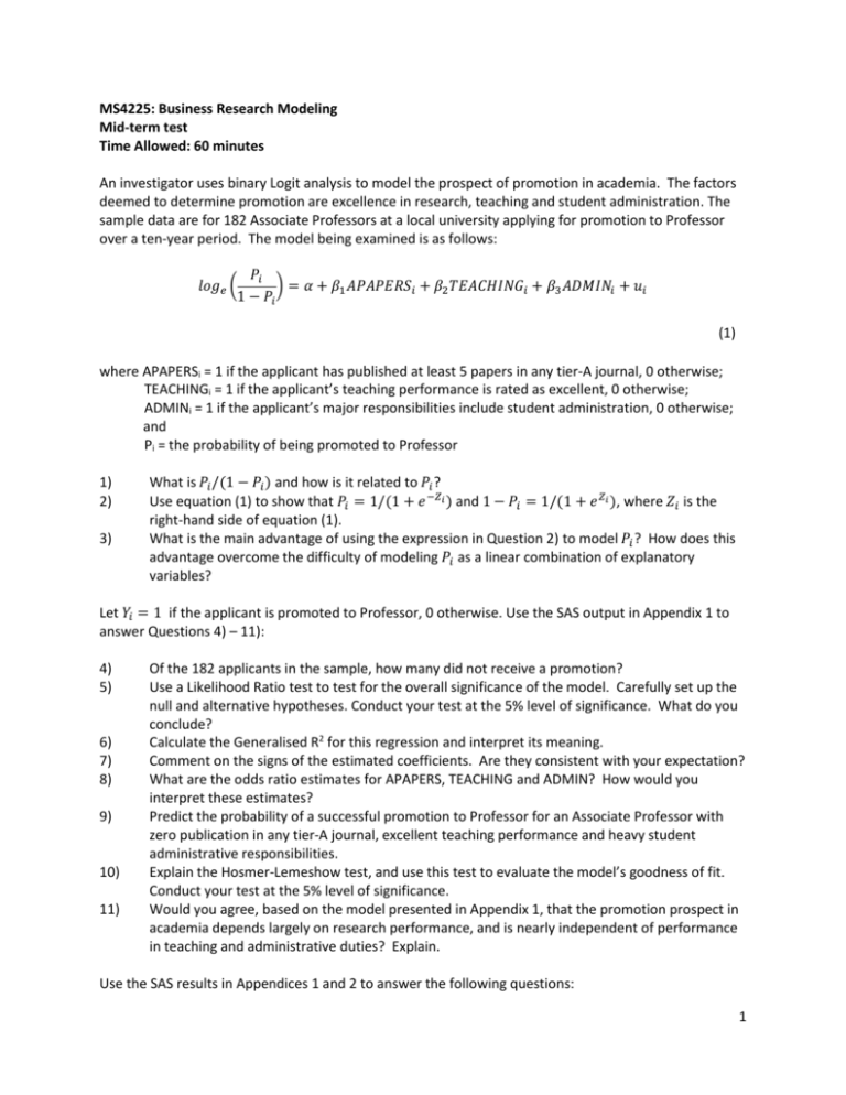
MS4225: Business Research Modeling
Mid-term test
Time Allowed: 60 minutes
An investigator uses binary Logit analysis to model the prospect of promotion in academia. The factors
deemed to determine promotion are excellence in research, teaching and student administration. The
sample data are for 182 Associate Professors at a local university applying for promotion to Professor
over a ten-year period. The model being examined is as follows:
𝑃𝑖
𝑙𝑜𝑔𝑒 (
) = 𝛼 + 𝛽1 𝐴𝑃𝐴𝑃𝐸𝑅𝑆𝑖 + 𝛽2 𝑇𝐸𝐴𝐶𝐻𝐼𝑁𝐺𝑖 + 𝛽3 𝐴𝐷𝑀𝐼𝑁𝑖 + 𝑢𝑖
1 − 𝑃𝑖
(1)
where APAPERSi = 1 if the applicant has published at least 5 papers in any tier-A journal, 0 otherwise;
TEACHINGi = 1 if the applicant’s teaching performance is rated as excellent, 0 otherwise;
ADMINi = 1 if the applicant’s major responsibilities include student administration, 0 otherwise;
and
Pi = the probability of being promoted to Professor
1)
2)
3)
What is 𝑃𝑖 /(1 − 𝑃𝑖 ) and how is it related to 𝑃𝑖 ?
Use equation (1) to show that 𝑃𝑖 = 1/(1 + 𝑒 −𝑍𝑖 ) and 1 − 𝑃𝑖 = 1/(1 + 𝑒 𝑍𝑖 ), where 𝑍𝑖 is the
right-hand side of equation (1).
What is the main advantage of using the expression in Question 2) to model 𝑃𝑖 ? How does this
advantage overcome the difficulty of modeling 𝑃𝑖 as a linear combination of explanatory
variables?
Let 𝑌𝑖 = 1 if the applicant is promoted to Professor, 0 otherwise. Use the SAS output in Appendix 1 to
answer Questions 4) – 11):
4)
5)
6)
7)
8)
9)
10)
11)
Of the 182 applicants in the sample, how many did not receive a promotion?
Use a Likelihood Ratio test to test for the overall significance of the model. Carefully set up the
null and alternative hypotheses. Conduct your test at the 5% level of significance. What do you
conclude?
Calculate the Generalised R2 for this regression and interpret its meaning.
Comment on the signs of the estimated coefficients. Are they consistent with your expectation?
What are the odds ratio estimates for APAPERS, TEACHING and ADMIN? How would you
interpret these estimates?
Predict the probability of a successful promotion to Professor for an Associate Professor with
zero publication in any tier-A journal, excellent teaching performance and heavy student
administrative responsibilities.
Explain the Hosmer-Lemeshow test, and use this test to evaluate the model’s goodness of fit.
Conduct your test at the 5% level of significance.
Would you agree, based on the model presented in Appendix 1, that the promotion prospect in
academia depends largely on research performance, and is nearly independent of performance
in teaching and administrative duties? Explain.
Use the SAS results in Appendices 1 and 2 to answer the following questions:
1
12)
13)
Use a Likelihood Ratio test to test for the joint significance of TEACHING and ADMIN on the
probability of receiving a promotion. Conduct your test at the 5% level of significance.
In your view, which of the two models in Appendices 1 and 2 is a superior model? Carefully
explain your answer.
Appendix 1
The LOGISTIC Procedure
Model Information
Data Set
Response Variable
Number of Response Levels
Number of Observations
Model
Optimization Technique
WORK.TEST
Y
2
182
binary logit
Fisher's scoring
Response Profile
Ordered
Value
Y
Total
Frequency
1
2
1
0
83
99
Probability modeled is Y=1.
Model Convergence Status
Convergence criterion (GCONV=1E-8) satisfied.
Model Fit Statistics
Criterion
AIC
SC
-2 Log L
Intercept
Only
Intercept
and
Covariates
252.897
256.101
250.897
85.771
98.587
77.771
Testing Global Null Hypothesis: BETA=0
Test
Chi-Square
DF
Pr > ChiSq
????????
141.5000
64.5709
3
3
3
<.0001
<.0001
<.0001
Likelihood Ratio
Score
Wald
The LOGISTIC Procedure
Analysis of Maximum Likelihood Estimates
Parameter
DF
Estimate
Standard
Error
Wald
Chi-Square
Pr > ChiSq
Intercept
1
-4.0731
0.8579
22.5432
<.0001
2
APAPERS
TEACHING
ADMIN
1
1
1
6.0149
1.0274
-0.1344
0.7771
0.7041
0.6347
59.9046
2.1291
0.0448
<.0001
0.1445
0.8323
Odds Ratio Estimates
Effect
Point
Estimate
APAPERS
TEACHING
ADMIN
95% Wald
Confidence Limits
????
????
????
89.274
0.703
0.252
>999.999
11.107
3.033
Association of Predicted Probabilities and Observed Responses
Percent Concordant
Percent Discordant
Percent Tied
Pairs
94.1
3.1
2.8
8217
Somers' D
Gamma
Tau-a
c
0.910
0.937
0.454
0.955
Partition for the Hosmer and Lemeshow Test
Group
Total
Observed
Event
Expected
1
2
3
4
5
6
7
8
20
18
25
31
21
21
24
22
0
0
2
1
18
19
22
21
0.29
0.30
1.00
1.41
18.04
18.37
22.67
20.93
Nonevent
Observed
Expected
20
18
23
30
3
2
2
1
19.71
17.70
24.00
29.59
2.96
2.63
1.33
1.07
Hosmer and Lemeshow Goodness-of-Fit Test
Chi-Square
DF
Pr > ChiSq
2.3117
6
0.8889
Appendix 2
The LOGISTIC Procedure
Model Information
Data Set
Response Variable
Number of Response Levels
Number of Observations
Model
Optimization Technique
WORK.TEST
Y
2
182
binary logit
Fisher's scoring
Response Profile
Ordered
Value
Y
Total
Frequency
3
1
2
1
0
83
99
Probability modeled is Y=1.
Model Convergence Status
Convergence criterion (GCONV=1E-8) satisfied.
Model Fit Statistics
Criterion
AIC
SC
-2 Log L
Intercept
Only
Intercept
and
Covariates
252.897
256.101
250.897
84.187
90.595
80.187
Testing Global Null Hypothesis: BETA=0
Test
Chi-Square
DF
Pr > ChiSq
170.7099
140.9750
67.7842
1
1
1
<.0001
<.0001
<.0001
Likelihood Ratio
Score
Wald
The LOGISTIC Procedure
Analysis of Maximum Likelihood Estimates
Parameter
DF
Estimate
Standard
Error
Wald
Chi-Square
Pr > ChiSq
Intercept
APAPERS
1
1
-3.4122
5.7148
0.5868
0.6941
33.8162
67.7842
<.0001
<.0001
Odds Ratio Estimates
Effect
Point
Estimate
APAPERS
303.315
95% Wald
Confidence Limits
77.814
>999.999
Association of Predicted Probabilities and Observed Responses
Percent Concordant
Percent Discordant
Percent Tied
Pairs
88.6
0.3
11.1
8217
Somers' D
Gamma
Tau-a
c
0.883
0.993
0.441
0.942
4