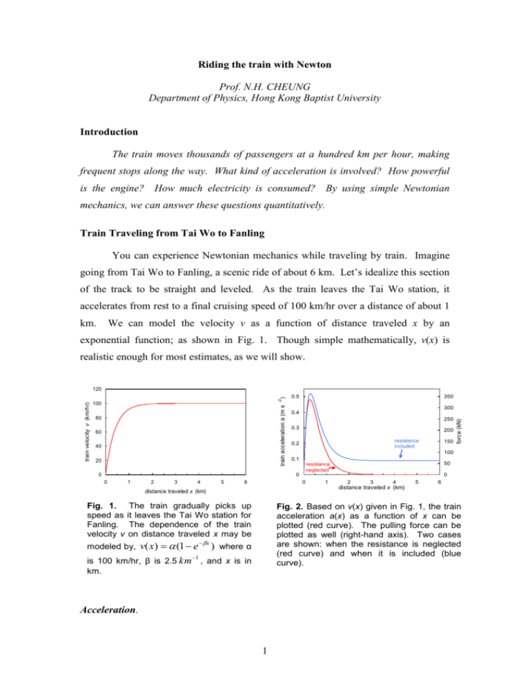
Riding the train with Newton
Prof. N.H. CHEUNG
Department of Physics, Hong Kong Baptist University
Introduction
The train moves thousands of passengers at a hundred km per hour, making
frequent stops along the way. What kind of acceleration is involved? How powerful
is the engine? How much electricity is consumed? By using simple Newtonian
mechanics, we can answer these questions quantitatively.
Train Traveling from Tai Wo to Fanling
You can experience Newtonian mechanics while traveling by train. Imagine
going from Tai Wo to Fanling, a scenic ride of about 6 km. Let’s idealize this section
of the track to be straight and leveled. As the train leaves the Tai Wo station, it
accelerates from rest to a final cruising speed of 100 km/hr over a distance of about 1
km.
We can model the velocity v as a function of distance traveled x by an
exponential function; as shown in Fig. 1. Though simple mathematically, v(x) is
realistic enough for most estimates, as we will show.
80
60
40
20
0.5
350
300
0.4
250
0.3
200
resistance
included
0.2
100
0.1
0
1
2
3
4
5
0
6
50
resistance
neglected
0
0
150
force (kN)
-2
100
train acceleration a (m s
train velocity v (km/hr)
)
120
1
0
2
3
4
5
6
distance traveled x (km)
distance traveled x (km)
Fig. 1. The train gradually picks up
speed as it leaves the Tai Wo station for
Fanling. The dependence of the train
velocity v on distance traveled x may be
Fig. 2. Based on v(x) given in Fig. 1, the train
acceleration a(x) as a function of x can be
plotted (red curve). The pulling force can be
plotted as well (right-hand axis). Two cases
are shown: when the resistance is neglected
(red curve) and when it is included (blue
curve).
v( x)   (1  e  x ) where α
1
is 100 km/hr, β is 2.5 km , and x is in
modeled by,
km.
Acceleration.
1
We will first calculate the acceleration a(x) as a function of x.
Using
elementary calculus, we have,
a
dv dv dx dv


v;
dt dx dt dx
(1)
so a(x) is simply the slope of the curve of v(x) vs x (Fig. 1) times the velocity. This is
plotted in Fig. 2 (red curve, left-hand axis). As can be seen, the train accelerates
maximally near the beginning, and soon travels at a constant velocity. The peak
acceleration is about 5% of the acceleration due to gravity, which is well within the
comfort zone of most people.
Start up power
We now estimate the force exerted by the engine to accelerate the train. There
are typically 12 carriages per train, each weighing about 40 metric ton when empty.
Loading capacity is about 300 passengers each. So the total mass is about 7  10 5 kg.
The start up force F(x) is simply the mass times the acceleration, which is depicted in
Fig. 2 (red curve, right-hand axis). Notice the start up force can be as high as 340 kN.
Two observations should be drawn. First, a train normally has four engines. Each
can exert a maximum pulling force of about 100 kN. So the train is working just
about as hard as it possibly can at start up. Second, the coefficient of friction between
the wheels and the railroad track is about 0.1 when cruising and increases to about 0.3
when stationary. Given a mass of 7  10 5 kg, the frictional drag (700 - 2,000 kN) is
certainly large enough to prevent slippage.
The work done dW by the engine is F dx. The mechanical power P expended
is dW/dt = F dx/dt = F v. This is plotted in Fig. 3 (red curve), as a function of x. The
maximum power drawn is about 5.5 MW, or about 7,400 horsepower.
This is
reasonable because we are transporting the mass equivalent of about 10 4 people.
Requiring 7,400 horses sounds about right.
2
engine power expended P (MW)
7
6
5
4
resistance
included
3
2
resistance
neglected
1
0
0
1
2
3
4
5
6
distance traveled x (km)
Fig. 3. The power expended P as a function of x. Two
cases are shown: when resistance is neglected (red
curve) and when it is included (blue curve).
Effortless cruising?
According to the red curve in Fig. 3, the engine can be turned off once the
train has reached its cruising speed of 100 km/hr. This is certainly unrealistic. Even
when the train is not accelerating, the engine still has to work hard to overcome all
kinds of mechanical friction, including bearing resistance of the moving parts and
wheel-track resistance. This mechanical resistance R m is found to increase with train
velocity. For local trains, R m (in N) may be modeled by a polynomial in v (in km/hr),
Rm (v )  10 4  130v  0.04v 2 . In addition to mechanical friction, there is air drag
as well. For still air, the aerodynamic resistance Ra (in N) varies approximately as
the square of the train velocity v (in km/hr), R a (v )  4v 2 . The total resistance R is
simply the sum of Rm and Ra,
R(v )  10 4  130v  4.04v 2 .
(2)
Therefore, the total force FT exerted by the engine is the sum of R and the
start-up force F(x). FT (x) is the blue curve shown in Fig. 2 (right-hand axis). As can
be seen, force against resistance is a minor component near start up, but becomes the
sole effort while cruising. Similarly, more power is expended when resistance is
taken into account, as depicted by the blue curve in Fig. 3.
3
Electricity bill
What is the cost of electricity to power this leg of the journey? Let’s calculate
6
the total work done. It is given by  FT dx , which is the area under the blue curve in
0
Fig. 2, or about 6  10 8 J. Assuming an efficiency of about 70 %, the total electrical
energy consumed is about 9  10 8 J. The cost of electricity (high power tariff) is about
$0.50 per kW-hr, so the electricity bill comes to about $125.
Enjoy your ride
Hopefully, you now appreciate how physics can help you estimate,
quantitatively, the key dynamical parameters of train motion based on just a few
assumptions. When you find the carriage lights dim or the air-conditioning weakens
as the train starts off at Tai Woo, you know the engine is pooling power to accelerate
the massive vehicle. And you know what percent of your train fare goes to paying the
electricity bill. Of course, you will find a lot more examples of Newtonian mechanics
around you. So by the time when you become the first astronaut from Hong Kong,
you know deep down that space travel is just one more application.
In the mean time, please relax and enjoy the rest of the scenic ride.
About the Author:
Prof. N.H. Cheung received his BA (Hons) degree in Physics from the University of
Chicago, and PhD degree in Physics from Cornell University. He is presently a
Professor of Physics at Hong Kong Baptist University. His research interests are in
laser-material interactions for analytical and biological applications.
Keywords:
Acceleration, velocity, power, force, friction
Glossary with pop-up explanation:
Horsepower, mechanical resistance, aerodynamic resistance, coefficient of
friction
Related Topics in the Syllabus:
Mechanics
Extensions(from the syllabus):
Bring out idea: From the graph of the article, we can find that most of the
energy is used to overcome friction (mechanical resistance and aerodynamic
resistance). Both resistances increase with velocity of trains.
4
Warm-up discussion:
 Try to search the travel time from Tai Woo to Fanling on the web and then
compare the time estimated in Fig 1.
 Using Fig. 1, compute the total time it takes to go from Tai Wo to Fanling. Is it
reasonable?
 Show that the area under the blue curve in Fig. 2 is 6 × 10 8 J.
Points for further discussion:







While cruising, the force exerted by the train is known to be about 60 kN. Is this
consistent with Fig. 2?
Given that the braking deceleration is about 0.9ms-2, calculate the stopping
distance and the time elapsed to bring a train from 100 km/hr to a complete
standstill. Are your results reasonable?
If the train travels up an incline of 1:100 (vertical:horizontal), how would the
electricity bill be different?
Is the meager electricity cost reasonable? Identify the other major costs in train
operation.
Is it possible for local trains to go at much higher speed, such as 200 km/hr?
What prevents it?
Last year, Shanghai’s first magnetic levitation train was launched. This kind of
train can go at very high speed, why? Discuss their working mechanism.
If the train ride is in space, how will the analysis be modified?
Activities:

Verification of the assumptions
Ride the train from Tai Wo to Fanling and see if the data used in this passage are
realistic or not. For example, design a practical method to measure v(x) of trains.
Measure the train velocity between Tai Wo and Fanling and plot a more realistic
Fig. 1. Based on your new Fig. 1, re-plot Figs. 2 and 3.

Similar ride
Do a similar analysis for MTR trips. What fraction of the fare goes to electricity?
Do it for long distance bus rides. What fraction of the bus fare goes to fuel cost?

Role Play
If you are the cost manager of KCR, based on the above passage, how would you
suggest ways to reduce running cost?

High Speed Trains
Look up the latest technological developments in mass transits, such as super
high speed trains. Identify interesting applications of physics principles. You
may even want to build a magnetically levitated model train using magnetized
strips and cardboard. A competition can be organized. The train that goes
farthest wins.
Related web sites:
5
o
o
o
o
o
KCR technology update
This site introduces the history and the future developments of KCR.
http://www.railway-technology.com/projects/kowloon/
Working of train wheels
This site gives a brief introduction on the history of railway and
information of the train wheels.
http://www.bbc.co.uk/science/hottopics/transport/railways.shtml
Magnetically levitated trains
This site introduces the magnetically levitated trains.
http://www.o-keating.com/hsr/maglev.htm
Contextual Physics
The section “Mechanics” in this site contains many information and
teaching materials of mechanics and trains.
http://www.phy.cuhk.edu.hk/contextual/
Physics World---MagLev
This site introduces the principle of magnetically levitated trains.
http://www.hk-phy.org/articles/maglev/maglev_e.html
References:
H.I. Andrews, Railway Traction: The Principles of Mechanical and Electrical Railway
Traction, especially Chapter 1 (Elsevier, Amsterdam, 1986).
6