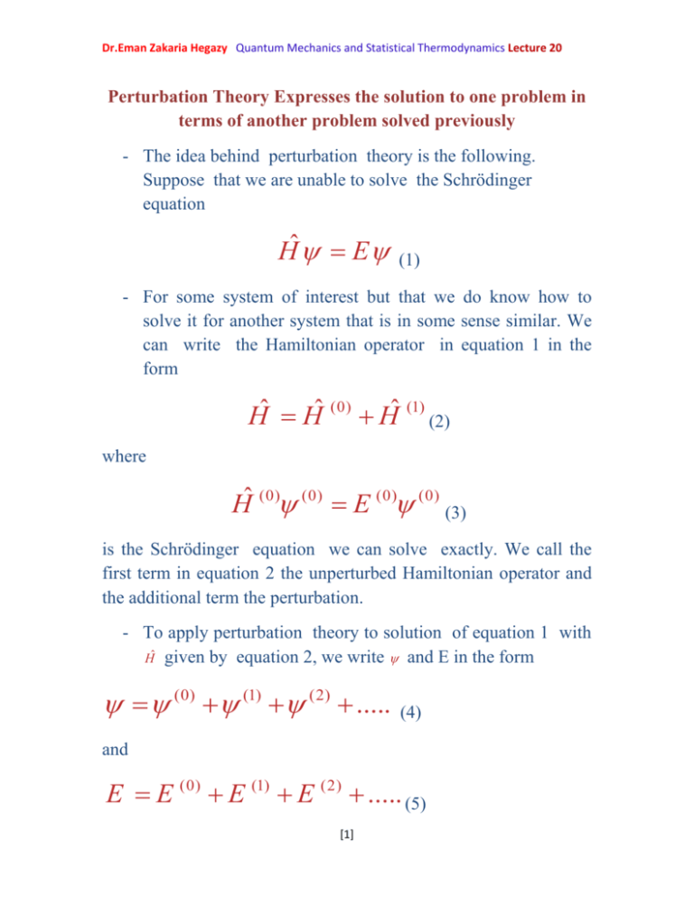
Dr.Eman Zakaria Hegazy Quantum Mechanics and Statistical Thermodynamics Lecture 20
Perturbation Theory Expresses the solution to one problem in
terms of another problem solved previously
- The idea behind perturbation theory is the following.
Suppose that we are unable to solve the Schrödinger
equation
Hˆ   E 
(1)
- For some system of interest but that we do know how to
solve it for another system that is in some sense similar. We
can write the Hamiltonian operator in equation 1 in the
form
Hˆ  Hˆ (0)  Hˆ (1) (2)
where
Ĥ (0) (0)  E (0) (0) (3)
is the Schrödinger equation we can solve exactly. We call the
first term in equation 2 the unperturbed Hamiltonian operator and
the additional term the perturbation.
- To apply perturbation theory to solution of equation 1 with
Hˆ given by equation 2, we write  and E in the form
   (0)  (1)  (2)  .....
(4)
and
E  E (0)  E (1)  E (2)  ..... (5)
[1]
Dr.Eman Zakaria Hegazy Quantum Mechanics and Statistical Thermodynamics Lecture 20
where  (0) and E(0) are given by the solution to unperturbed
problem equation (3) and  (1) , (2) ,..... are successive correction to
 (0) and E(1), E(2),…. are successive corrections to E(0). A baic
assumption is that theses successive corrections become
increasingly less significant. Although we will not do so here, we
can derive explicit expressions for these corrections. The only one
we will use is the expression for E(1) , which is
E (1)   (0)*Hˆ (1) (0)d 
(6)
we say that E(1) is the first –order correction to E(0) , and we write
E  E (0)  E (1) (7)
Equation 7 represents the energy through first order perturbation
theory. If we were to evaluate  (1) (which we will not), then
   (0)  (1) (8)
Would represent  through first order. Similarly, if we were to
evaluate E (2) (which we will not), then
E  E (0)  E (1)  E (2)
Would represent E through second order perturbation theory. In
this book, we evaluate E to first order only, using equation 6.
[2]
Dr.Eman Zakaria Hegazy Quantum Mechanics and Statistical Thermodynamics Lecture 20
Perturbation theory to calculate the energy of a particle in box
- We will use first order perturbation theory to calculate the
energy of a particle in box from x=0 to x=a with a slanted
bottom, such that
V (x ) 
V 0x
a
0x a
In this case, the unperturbed problem is a particle in a box and so
V x
Hˆ (1)  0
a
0x a
Where V0 is a constant. The wave functions and the energies for a
particle in a box are
n x
2
   sin
a
a 
12
 (0)
0x a
and
E
(0)
n 2h 2

8ma 2
According to equation 6 , the first order correction of E(0) due to
perturbation is given by
V

  (0)*  0 x   (0) dx
a 
0
a
E
(1)
2V 0
2 n x
x
sin
dx
a 2 0
a
a
=
[3]
Dr.Eman Zakaria Hegazy Quantum Mechanics and Statistical Thermodynamics Lecture 20
This integral occurs previously and is equal to a2/4. Therefore, we
find that
E (1) 
V0
2
For all values of n. the energy levels are given through first order
by
n 2h 2 V 0
2
E 
+
+O(V
) n=1,2,3,....
0
2
8ma
2
Where the term O (V02) emphasizes that terms of order V02 and
higher have been dropped. Thus, we see in this case that each of
the unperturbed energy levels s shifted by V0/2.
[4]
Dr.Eman Zakaria Hegazy Quantum Mechanics and Statistical Thermodynamics Lecture 20
Helium atom
- We can apply perturbation theory to the helium atom whose
Hamiltonian operator is given by equation
2
2
2
2
e
1
1
e
1
Hˆ  
(   ) 
(  )
2m e
4 0 r1 r2 4 0 r12
2
1
2
2
For simplicity we will consider only the ground –state energy. If
we consider the interelectronic repulsion term
e2
4 0 r12
, to be the
perturbation , then the unperturbed wave fnctions and energies
are the hydrogenlike quantities given by
Hˆ (0)  Hˆ (1)  Hˆ (2)
 (0)   1s (r1 ,1 , 1 ) 1s (r2 , 2 , 2 )
E
(0)
(9)
Z 2 mee 4
Z 2 mee 4


32 2 0 2 n12 32 2 0 2 n 22
and
Hˆ (1) 
e2
4 0 r12
with Z= 2. Using Equation (6), we have
E
(1)
  dr1dr2 1s (r1 ) 1s (r2 )
where
[5]
e2
 1s (r1 ) 1s (r2 ) (10)
4 0 r12
Dr.Eman Zakaria Hegazy Quantum Mechanics and Statistical Thermodynamics Lecture 20
1/2
 Z3 
 zr / a
 1s (r j )   3  e j 0
 a0  
The final result is that
E (1) 
5Z
8
 me e 4

2 2
 16  0
2



(11)
1
1
5
E  E (0)  E (1)   Z 2  Z 2  Z
2
2
8
5
 Z 2  Z
8
(12)
- Letting Z= 2 gives -2.750 compared with our simple
variational result (-2.8477) and the experimental results of 2.9033.
- So we see that first order perturbation gives a result is about
5% in error. It turns out that second order perturbation theory
gives -2.910
- Thus, we see that both the variational method and the
perturbation theory are able to achieve very good results.
[6]