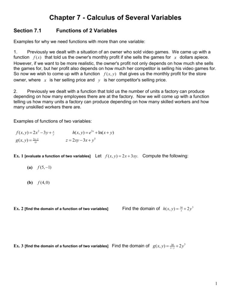
Chapter 7 - Calculus of Several Variables
Section 7.1
Functions of 2 Variables
Examples for why we need functions with more than one variable:
1.
Previously we dealt with a situation of an owner who sold video games. We came up with a
function f ( x) that told us the owner's monthly profit if she sells the games for x dollars apiece.
However, if we want to be more realistic, the owner's profit not only depends on how much she sells
the games for, but her profit also depends on how much her competitor is selling his video games for.
So now we wish to come up with a function f ( x, y ) that gives us the monthly profit for the store
owner, where x is her selling price and y is her competitor's selling price.
2.
Previously we dealt with a function that told us the number of units a factory can produce
depending on how many employees there are at the factory. Now we will come up with a function
telling us how many units a factory can produce depending on how many skilled workers and how
many unskilled workers there are.
Examples of functions of two variables:
f ( x, y)  2 x2  3 y  xy
g ( x, y)  3xxy1
h( x, y)  e3x  ln( x  y)
z  2 xy  3x  y5
Ex. 1 [evaluate a function of two variables] Let f ( x, y )  2 x  3 xy. Compute the following:
(a)
f (5, 1)
(b)
f (4, 0)
Ex. 2 [find the domain of a function of two variables]
Find the domain of h( x, y )  30x  2 y 3
Ex. 3 [find the domain of a function of two variables] Find the domain of g ( x, y) 
30
x y
 2 y3
1
Ex. 4 [find a change in a quantity] Using x skilled workers and y unskilled workers, a manufacturer
can produce Q( x, y)  10 x 2 y units per day. Currently there are 20 skilled workers and 40
unskilled workers on the job.
(a) How many units are currently being produced?
(b) By how much will the daily production level change if 1 more skilled worker is added to the
current workforce?
(c) By how much will the daily production level change if 1 more unskilled worker is added to
the current workforce?
Graphs of functions of 2 variables:
2
Consider a hiker in the mountains. Since a 3D model of the mountain isn’t practical to carry around,
the hiker carries a topographical map. For various heights, a slice of the mountain is taken and placed
on the map. These “rings” on the map indicate areas of equal elevation.
Curves like this are sometimes put on a weather map, to indicate places where the temperatures are
the same. In this context, the level curve is called an isotherm.
This idea can be used to draw a graph for any function of two variables z  f ( x, y ) . The mathematical
equivalent to a curve on a topographical map is called a level curve of f ( x, y ) .
3
Ex. 5 [draw level curves] Let f ( x, y)  x 2  6 x  y. Draw the level curves, f ( x, y )  C , for each of the
following cases:
(a) C  0
(b) C  5
(c) C  7
4
Some Economic Interpretations of Level Curves
If Q ( x, y ) measures the output of a production process, then a level curve Q ( x, y )  C is called a
"curve of constant product C ".
If U ( x, y ) is a utility function which measures the total satisfaction (utility) the consumer derives from
have x units of the first commodity and y units of the second, then a level curve U ( x, y )  C is
called an indifference curve (this curve gives all the combinations of x and y that lead to the same
level of consumer satisfaction.)
Ex. 6 [determine level of utility]; [sketch indifference curve] Suppose the utility derived by a consumer
from x units of one commodity and y units of a second commodity is given by the utility function
U ( x, y)  x3/2 y. If the consumer currently owns 16 units of the first commodity and 20 units of the
second, find the consumer's current level of utility and sketch the corresponding indifference curve.
5
Section 7.2
Partial Derivatives
Just like we did with functions of one variable, we will now want to take derivatives of functions with
two variables.
How do we take a derivative of f ( x, y)  x 21  3 y 4  x 2 y 5 ?
1 st : Consider f as only a function of x. (ie. y is held fixed at some number: y does not
change!) Now take the derivative of f with respect to the only variable, x.
This is called the derivative of f ( x, y ) with respect to x .
We write f x ( x, y )  21x 20  2 xy 5
Or simply f x  21x 20  2 xy 5
2 nd : Consider f as only a function of y. (ie. x is held fixed at some number -- x does not
change!) Now take the derivative of f with respect to the only variable -- y.
This is called the derivative of f ( x, y ) with respect to y .
We write f y ( x, y)  12 y3  5x2 y 4
Or simply f y  12 y3  5x2 y 4
Alternate notation: If we write z  x 21  3 y 4  x 2 y 5 then
20
z
 2 xy 5
x  21x
z
y
 12 y3  5x2 y 4
6
Ex. 1 [find partial derivatives] f ( x, y)   x 2  2 xy  1 .
5
Ex. 2 [find partial derivatives] z  ye x
2
1
Ex. 3 [find partial derivatives] h( x, y) 
 ln y  1x .
x2 1 .
y 2
Compute f x
Compute xz
Compute hx
and
and
fy
z .
y
and hy .
7
Ex. 4 [find partial derivatives] z  ln( x 2 y )  xy .
Compute xz
and
z .
y
Recall that the derivatiive of f ( x) gives a rate of change of f ( x) (how quickly f is changing).
f x and f y give rates of change also.
fx
= how quickly f is changing with respect to x
= how quickly f is changing if we hold y constant and let x vary.
fy
= how quickly f is changing with respect to y
= how quickly f is changing if we hold x constant and let y vary.
Ex. 5 [interpret economic meaning of partial derivative] Suppose that a store's monthly demand for a
computer game is given by h( x, y ) , where x is the store's price of the game and y is the
competitor's price of the same game. Under normal economic conditions what should the signs of hx
and hy be?
8
Approximations Using Partial Derivatives
Recall our approximation formula for functions of one variable:
f  f  ( x) x
We have two approximation formulas for functions with two variables:
1. If y remains constant then f ( x, y ) is really just a function of x, and thus
f ( x, y)  f x x
2. If x remains constant then f ( x, y ) is really just a function of y, and thus
f ( x, y )  f y y
Ex. 6 [approximate change using partial derivatives] A manufacturer estimates that the annual output at
a certain factory is given by Q( K , L)  30K 0.3 L0.7 units, where K is the capital expenditure in units
of $1, 000 and L is the size of the labor force in worker-hours. The current levels are $630, 000 of
capital investment and 830 worker-hours of labor.
(a)
Determine the marginal productivity of capital (the change in output due to an additional
unit of $1, 000 of capital expenditure).
(b)
Determine the marginal productivity of labor (the change in output due to an additional
unit of 1 worker-hour of labor).
(c)
Should the manufacturer consider adding a unit of capital or a unit of labor in order to
increase output more rapidly?
9
Second Derivatives
Alternate notation:
z
f ( x, y )
Function
------------------------------------------------------------z
1 st Derivatives
fx
x
z
fy
y
-----------------------------------------------------------2 z
2 nd Derivatives
f xx
x 2
f xy
2 z
xy
f yx
2 z
yx
f yy
2 z
y 2
Ex. 7 [find second partial derivatives] Find all the second derivatives of f ( x, y)  x 2 y  x5 y 4  2 y  x 2
Answer:
f xx 
f xy 
f yx 
f yy 
10
Section 7.3
Optimization
For a point to be a relative minimum
or a relative maximum,all tangent lines
must be horizontal. This means that
both f x AND f y must be 0.
Unfortunately, having f x  0 and
f y  0 does not guarentee that a
relative maximum or relative
minimum is produced.
Recall one of our methods to find the relative extrema of f(x) was:
1. Find the critical values (Solve the equation f  ( x)  0 ).
2. Use the 2 nd Derivative Test to determine which numbers in step 1 are relative
maximums, which are relative minimums, and which are neither.
We shall continue to do this for functions of two variables, with a few minor adjustments.
11
Definition of a critical point:
(a, b) is a critical point of f ( x, y ) if
Theorem (2
nd
f x (a, b)  0
and
f y (a, b)  0.
Partials Test):
2
Suppose (a, b) is a critical point of f ( x, y ). Let D  f xx f yy   f xy  , evaluated at the point
(a, b).
(a) If D  0 then f has a saddle point at (a, b) .
(b) If D  0 and f xx (a, b)  0 then f has a relative maximum at (a, b) .
(c) If D  0 and f xx (a, b)  0 then f has a relative minimum at (a, b) .
Ex. 1 [find critical points for function of two variables]; [classify critical points] Find all the critical points of
f ( x, y)  100  x 2  y 2 and classify them.
Ex. 2 [find critical points for function of two variables]; [classify critical points] Find all the critical points of
g ( x, y)  2 x3  y 3  3x 2  3 y  12 x  4 and classify them.
12
Ex. 3 [find critical points for function of two variables]; [classify critical points] Find all the critical points
of f ( x, y)   x3  y 3  3xy and classify them.
In the word problems we'll be asked to optimize some quantity (i.e. - minimize costs, maximize volume, maximize profit,
and so on.). But this is asking for absolute extrema, not relative extrema (and we've only considered relative extrema).
No problem though -- in all the word problems we'll see in this section, relative extrema are also absolute extrema.
Ex. 4 [solve a practical optimization problem]The only grocery store in a small rural community carries
two brands of frozen apple juice, a local brand that it obtains at a cost of 30 cents per can and a wellknown national brand that it obtains at the cost of 40 cents per can. The grocer estimates that if the
local brand is sold for x cents per can and the national brand for y cents per can, approximately
70  5 x  4 y cans of the local brand and 80  6 x  7 y cans of the national brand will be sold each
day. How should the grocer price each brand to maximize the profit from the sale of the juice?
13
Math 143
Chapter Seven
List of Procedures
7.1
evaluate a function of two variables
find the domain of a function of two variables
find a change in a quantity
draw level curves
determine level of utility
sketch indifference curve
7.2
find partial derivatives
interpret economic meaning of partial derivative
approximate change using partial derivatives
find second partial derivatives
7.3
find critical points for function of two variable
classify critical points
solve a practical optimization problem
14