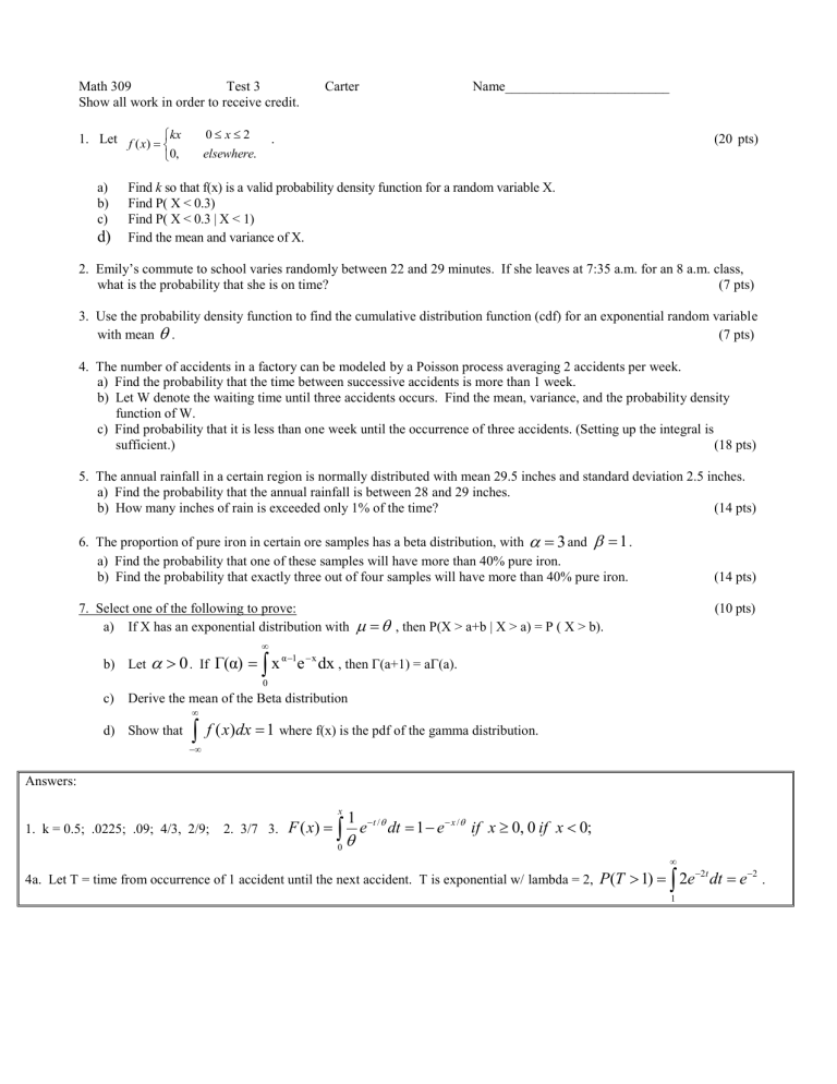
Answers:
Math 309 Test 3
Show all work in order to receive credit.
Carter Name________________________
1. Let
 kx 0 2
.
 0, elsewhere .
a) Find k so that f(x) is a valid probability density function for a random variable X. b) Find P( X < 0.3) c) Find P( X < 0.3 | X < 1)
(20 pts) d) Find the mean and variance of X.
2. Emily’s commute to school varies randomly between 22 and 29 minutes. If she leaves at 7:35 a.m. for an 8 a.m. class, what is the probability that she is on time? (7 pts)
3. Use the probability density function to find the cumulative distribution function (cdf) for an exponential random variable with mean

. (7 pts)
4. The number of accidents in a factory can be modeled by a Poisson process averaging 2 accidents per week. a) Find the probability that the time between successive accidents is more than 1 week. b) Let W denote the waiting time until three accidents occurs. Find the mean, variance, and the probability density function of W. c) Find probability that it is less than one week until the occurrence of three accidents. (Setting up the integral is sufficient.) (18 pts)
5. The annual rainfall in a certain region is normally distributed with mean 29.5 inches and standard deviation 2.5 inches. a) Find the probability that the annual rainfall is between 28 and 29 inches. b) How many inches of rain is exceeded only 1% of the time?
6. The proportion of pure iron in certain ore samples has a beta distribution, with
 
3 and
 
1 .
(14 pts) a) Find the probability that one of these samples will have more than 40% pure iron. b) Find the probability that exactly three out of four samples will have more than 40% pure iron.
7. Select one of the following to prove: a) If X has an exponential distribution with
  
, then P(X > a+b | X > a) = P ( X > b).
(14 pts)
(10 pts) b) Let
 
0 . If
Γ(α) 


0 x
α 
1 e
 x dx , then

(a+1) = a

(a). c) Derive the mean of the Beta distribution d) Show that




1
where f(x) is the pdf of the gamma distribution.
1. k = 0.5; .0225; .09; 4/3, 2/9; 2. 3/7 3.
  x
0
1
 e
 t /
 dt e
 x /
 if x

0, 0 if x

0;
4a. Let T = time from occurrence of 1 accident until the next accident. T is exponential w/ lambda = 2,

(
 
2

2 t e dt
 e
1
 
2
.






1
 3
(3)(.5 )
0 x

0
2

2 x e x
4b. W is gamma w/ s = 3 and lambda = 2,
 
3 / 2;

2 
3
4
1
2

2 x c ) 4 x e dx
0
 x

0
5a) P(28 < X < 29) = P( -.6 < Z <-.2) = P(.2 < Z <.6) = .2257 - .0793 = .1464; 2.33 = (x – 29.5)/2.5 => x = 35.325
6a)

1
0.4

(4)
2 x dx

.936
; b) C
3
(4,3)(.936) (.064)
1 
.2099
Show all work in order to receive credit.
11/29/01
1. Consider a die with three equally likely outcomes. A pair of such dice is rolled. Let X denote the sum on the pair of dice and Y denote the “larger” number. The joint probability distribution is in the chart. a) P(X

4, Y

2) b) P( X = 4) c) P(X

4) d) P(Y = 2 | X = 4)
2. Consider the joint density function: g ( x , y )

6
0 x 0
 x

1 , 0 elsewhere .
 y

1 , 0
 x
 y

1 a) Find P(X < ¾, Y < ¼). b) Find P(X < ¾, Y < ½). c) Find P(X < ¾ | Y < ½). d) Find the conditional density function for X given Y = 1/2. e) Find P(X < 3/4 | Y = 1/2 ).
3. Consider the joint density function:
(
,
)



 0

( x
 y ) a) Find the marginal density functions f x
(x) and f y
(y). b) Are X and Y independent? Justify. c) Find P( X < Y) . (Set-up is sufficient.) d) Set-up an integral that gives E[X-Y].
0

 
.
, 0

 
4. Two friends are to meet at a library. Each arrives randomly at an independently selected time within a fixed one-hour period and agrees to wait no longer than 15 minutes for the other. Find the probability that they will meet. (Set up is sufficient.)
5. Explain the statement, “While covariance measures the direction of the association between two random variables, the correlation coefficient measures the strength of the association." Examples are appropriate in your comments.
6. Select one of the following. a) For either the discrete or continuous case, show that if X and Y are independent, E[XY] = E[X]E[Y]. b) Show that if X and Y are independent, Cov(X, Y) = 0. (Assume (a) & use the definition, Cov(X,Y) = E[(X-
 x c) Let Y
1
, Y
2
, …, Y n
be independent random variables with E(Y
E[X] = n
 and V(X) = n

2 where X = Y
1
+ Y
2
+ … + Y n
.
I
) =
 and V(Y
I
) =

2 . Show
) (Y-
 y
)].)

Answers/Solutions : For some I have given answers. Others have an intermediate step in the solution as I felt it would be more beneficial than just the answer. If you detect errors, please send an e-mail.
1. You need to know about the die. Assume that the die has two 1’s, two 2’s and two 3’s.
X
2 3 4 5 6
Y
1 1/ 9 0 0 0
2 0 2 / 9 1/ 9 0
0
0
3 0 0 2 / 9 2 / 9 1/ 9
5/9, 3/9, 6/9, 1/3
2a.
1/ 4 3/ 4
 
0 0
6 x dx dy b.
1/ 4 3/ 4
 
0 0
6

1

1/ 2
  y
1/ 4 0
6
c. answer from b
1/ 2

 f
2
( )

46 / 64
1/ 2

0
3(1

)
2 y dy
 d. f ( |

1/ 2)

46 / 64

46 / 56
7 / 8 f
2
(1/ 2)


6 x
2

8 x 0 1/ 2 e.
1/ 2

0
8 x dx

1
3a.
f x
1
 e
 x x

0; f
2
( )
 e
 y y b. X and Y are independent since

0
1
( )
2
( )
 x e e
 y  e c.

 y
0 0 x y )
d. [

Y ]

 

0 0
( x

) x y ) dx dy x y ) 
.
4. 1


 y
1
 
1/4 0

1
4
1

1/4 1
0
 
1 y

4
1



7
16
5. If Cov (X, Y) > 0, then as x increases, y increases. If Cov(X, Y) < 0 then as x increases, y decreases.
The correlation is standardized,
1

1
. If
|
 
then X & Y are perfectly linearly related – one can be thought of as a linear function of the other. When |

| is close to 1, the linearly correlation is strong. As
|

| gets closer to zero, the correlation is weak.

Fall 2011
The tests above do not have anything on moment generating functions or when we created new random variables by adding know random variables (e.g. Jack & Jill’s bowling scores). Study the assigned hw problems!
Chapter 7 – Expectations - Notes.
  y x
for a joint discrete distribution.

 
 
  for a joint continuous distribution.
E[aX + bY] = aE[X] + bE[Y] where E[X] and E[Y] are both finite. (This generalizes to the sum of n random variables.)
Cov ( X , Y )


E [( X
E [ XY

]


X

X
)( Y

Y
 
Y
)]
Note that if X & Y are independent, Cov(X, Y) = 0
Var(aX + bY) = a 2 Var(X) + b 2 Var(Y) – 2Cov(X, Y)
Note that if X & Y are independent the variance of their sum is the sum of their variances.
Moment Generating Functions (mgf), M(t) –
Know the definition - M(t) = E[e tx ];
Be able to derive mgf for binomial, Poisson, geometric, uniform continuous, exponential r.v.s;
Know how to find the moments of the r.v. from the mgf;
Know how to find the mean & variance of a r.v. from M(t).
The mgf uniquely defines the distribution – so if a mgf has the form of one of our known mgf, then you can find the associated probabilities, etc.
M
X+Y
(t) = M x
(t)M
Y
(t)
We used this to show that: the sum of r.v.’s with normal distributions is normal, the sum of r.v.’s with Poisson distributions is Poisson, the sum of r.v.’s with gamma distributions is gamma.
However, this is not true for the sums of all distributions. We used the relationship between mgf’s to show that the sum of r.v.’s with a uniform distribution is not uniform.