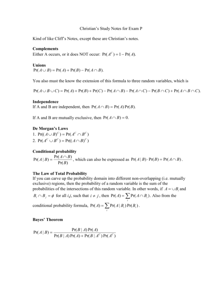
Christian’s Study Notes for Exam P
Kind of like Cliff’s Notes, except these are Christian’s notes.
Complements
Either A occurs, or it does NOT occur: Pr( AC )  1  Pr( A).
Unions
Pr( A  B )  Pr( A)  Pr( B )  Pr( A  B ).
You also must the know the extension of this formula to three random variables, which is
Pr( A  B  C )  Pr( A)  Pr( B )  Pr(C )  Pr( A  B )  Pr( A  C )  Pr( B  C )  Pr( A  B  C ).
Independence
If A and B are independent, then Pr( A  B )  Pr( A) Pr( B ).
If A and B are mutually exclusive, then Pr( A  B )  0.
De Morgan’s Laws
1. Pr(( A  B)C )  Pr( AC  B C )
2. Pr( AC  B C )  Pr(( A  B) C )
Conditional probability
Pr( A  B )
, which can also be expressed as Pr( A | B )  Pr( B )  Pr( A  B ) .
Pr( A | B ) 
Pr( B )
The Law of Total Probability
If you can carve up the probability domain into different non-overlapping (i.e. mutually
exclusive) regions, then the probability of a random variable is the sum of the
probabilities of the intersections of this random variable. In other words, if A   Bi and
Bi  B j   for all i,j, such that i  j , then Pr( A)   Pr( A  Bi ) . Also from the
i
conditional probability formula, Pr( A)   Pr( A | Bi ) Pr( Bi ) .
i
Bayes’ Theorem
Pr( A | B ) 
Pr( B | A) Pr( A)
Pr( B | A) Pr( A)  Pr( B | AC ) Pr( AC )
Expected Value
There are two ways to calculate the expected value. The basic, most direct route is one of
the things you have to know:
For a discrete distribution f(x),
E( X ) 

 x  f ( x)
x  
For a continuous distribution:

E( X ) 
 x  f ( x)dx

But there’s also another way to calculate the expected value that can be faster, based on
the information you are given in the problem.
For a discrete distribution:
E( X ) 

 Pr( X  x )
x  
For a continuous distribution,

E ( X )   Pr( X  x)dx

where Pr( X  x )  1  F ( x ) , where F is the cumulate distribution function.
You have to know the basic way to calculate the expected value; the other method is also
nice to know and can save you valuable time in the heat of the exam.
Variance
The variance of a random variable X, denoted Var(X), is given by the formula
Var( X )  E ( X 2 )  E ( X ) 2
Covariance
The covariance between two variables is Cov( X , Y )  E ( XY )  E ( X ) E (Y ) .
Also, you need to know that Var( X  Y )  Var( X )  Var(Y )  2Cov( X , Y ), and that
Var(aX  b)  a 2Var( X ) and Cov( aX , bY )  abCov( X , Y ).
The standard deviation, denoted  X , is simply the square root of the variance,
 X  Var( X ) .
Coefficient of variation: This is simply the ratio of the standard deviation to the mean,
that is
X
E( X )
.
Double Expectation
E(X) = EY(E(X|Y=y))
Var(X)=VarY(E(X|Y=y))+EY(Var(X|Y=y))
Wasn’t on my exam, but you never know.
Probability Distributions
Mean, median, and mode
The three most tested probability distributions are the uniform, exponential, and Poisson.
You also need to know the binomial, geometric, the negative binomial, and the
hypergeometric.
The Uniform Distribution
This is the simplest of the continuous distributions. You are given an interval (a,b), for
which the likelihood of any point in the interval is just as a likely as any other. The
1
probability density function is f ( x ) 
.
ba
b  a  .
ab
and the variance is
2
12
2
The mean of the uniform is
The Poisson Distribution
The Poisson distribution is used to model waiting times.
The important stuff:
The mean = 
The variance = 
The mode is equal to lambda, rounded down to the nearest integer. For example, a
Poisson distribution with mean equal to 3.2 has a mode equal to 3. A Poisson with mean
equal to 3 also has mode equal to 3.
Also good to know is that the sum of two Poisson distributions with means 1 and 2 is a
Poisson distribution with mean = 1 + 2.
It gets a little trickier if two Poisson distributions or more are involved. A shortcut that
can save you a significant amount of time is recognizing that the sum of two or more
Poisson distributions is also a Poisson distribution. For example, supposed that you are
asked the following question:
A business models the number of customers for the first week of each month as a Poisson
distribution with mean = 3, and for the second week of each month as a Poisson
distribution with mean = 2. What is the probability of having exactly two customers in
the first two weeks of a month? The long way to do this is to figure out all the different
combinations –
Case I – one customer in week one, one customer in week two.
Case II – two customers in week one, no customers in week two.
Case III – no customers in week one, two customers in week two.
The easy way to do this is to use the fact that the sum of two Poisson distributions is also
Poisson. So the sum of the Poisson distributions from weeks one and two is Poisson with
52 e 5
 0.084.
mean = 5. The probability of exactly two customers is
2!
The Exponential Distribution
This is another of the essential distributions. The exponential distribution is used to
measure the waiting time until failure of machines, among other applications.
f ( x )  e  x
The mean equals
1
, and the variance equals
1
. This is an important distinction from

2
the Poisson, where the mean is equal to the variance. For the exponential, the mean is
equal to the standard deviation, so the variance is equal to the mean squared.
Some useful integration shortcuts that can save you valuable time on the exam:

1
 e

x

dx  e

a

a

x
a
1


x
a
2

x
e  dx  (a   )e
1



a

x
e dx  (( a   )   ) e

2
2

a

The Gamma Distribution
It’s good to have a passing familiarity with the Gamma distribution. The sum of
exponential distributions is a gamma distribution. The exponential distribution is tested
very heavily on the exam, and there has been at least one recent exam question where it
would have been helpful to know that the sum of two exponentials is a gamma. That’s
about all you’ll need to know, but you might get tested on the gamma outright, so listed
below are some relevant formulas for the gamma. If pressed for time, skip this and focus
on the basics instead.
x

1
 1 
Gamma pdf: f ( x )  
x e
 ( )
The Bernoulli Distribution
Discrete distribution, the simplest probability distribution, either an event occurs, or
doesn’t occur. A probability is given for the event that the probability occurs.
1 with prob. p

X 

0 with prob.1  p  q 
E(X) = p
Var(X) = p(1-p)
Binomial Distribution
f (n, k , p)  C (k , n) p k (1  p) nk where C (k , n ) 
n!
.
k! (n  k )!
Mean = np, Variance = np(1-p)
Geometric Distribution
Perform Bernoulli trials until success, then stop and count the total number of trials – this
is the geometric random variable.
The tricky part about this is that there can be two different formulations, based on
whether you count the number of trials before the first success, or the number of failures
before the first success.
X = # trials until first success:
f X ( n )  (1  p ) n 1 p
E( X ) 
1
p
Var ( X ) 
1
1

2
p
p
Y = # failures before first success:
f Y ( k )  (1  p ) k p
1
1
p
1
1
Var (Y )  2 
p
p
E (Y ) 
Negative Binomial Distribution
k
f NB ( n, k , p )  f B ( n, k , p )
n
E (n) 
k
p
 1
1
Var(n )  k  2  
p
p
Hypergeometric Distribution
Used for sampling without replacement. Finite population with n objects, k are special, nk are not. If m objects are chosen at random, the probability that out of m, x are special is
k!
( n  k )!
x! ( k  x )! ( m  x )! ( n  k  ( m  x ))!
f ( x) 
n!
m! ( n  m )!
It looks a little complicated but once you’ve worked several problems, this is not too
hard.
Normal Distribution
Continuity correction factor for binomial or Poisson or uniform approximations:
 k  0.5   
 k  0.5   
Pr( X  k )  Pr( k  0.5  Y  k  0.5)   
  







Bivariate Normal Distribution

E (Y | X  x )  E (Y )   Y ( X  E ( X ))
X
 Y2|X  x  (1   2 ) Y2
Lognormal Distribution
 ln y  ln y
F ( y )  Pr(Y  y )  Pr(ln Y  ln y )   
 
ln y





1
E (Y )  e
2
ln y   ln
y
2
 2

Var(Y )  E (Y ) 2  e ln y  1


Other distributions on the syllabus include the beta, the Pareto, the Chi-Square, and the
Weibull. I have not presented them here.
Marginal Density
f ( x )   f ( x, y )dy
Y |X
Order Statistics
f X ( k ) ( x)  nf ( x)C(k  1, n  1) F ( x) k 1 (1  F ( x)) nk
Conditional Density
f ( x, y )
f X |Y ( x | y ) 
f ( y)
E (Y | X  x ) 
y f
Y |X
( y | x )dy
Y |X
Moment Generating Functions
MX(t)=E(etX)
MaX(t)=MX(at)
Mb(t)=ebt
X,Y independent => MX+Y(t)=MX(t)MY(t)
MX(0)=1
MGF for Bernoulli: pet+q
MGF for Binomial: (pet+q)n
t
MGF for Poisson: M X (t )  e  ( e 1)
1 2
MGF for Standard Normal: M X (t )  e 2
MGF for Normal: M X (t )  e
MGF for Exponential:
t
 t  12 2t 2
1
1 t
 1 

MGF for Gamma: 
1   t 
n
Note that based on a comparison of the MGFs for the exponential and gamma
distributions, it’s easy to see that the gamma is the sum of n exponential distributions.
Joint MGFs:
M X ,Y ( s, t )  E  e sX  tY 


E X nY m  
 nm
M X ,Y 0,0
 n s m t
A couple of other important formulas that can come in handy:
M X ,Y ( s,0)  M X ( s )
M X ,Y (0, t )  M Y (t )
M X ,Y ( s, t )  M X Y (t )
Chebyshev’s Theorem
Pr | X   |  c  
2
c
Benefit Distributions
E(X) = qE(B)
Var(X) = qE(B) – (qE(B))2
Miscellaneous Formulas
Kth central moment of X : E((X-E(X))k)
Correlation coefficient:  ( X , Y ) 
Cov( X , Y )
 XY