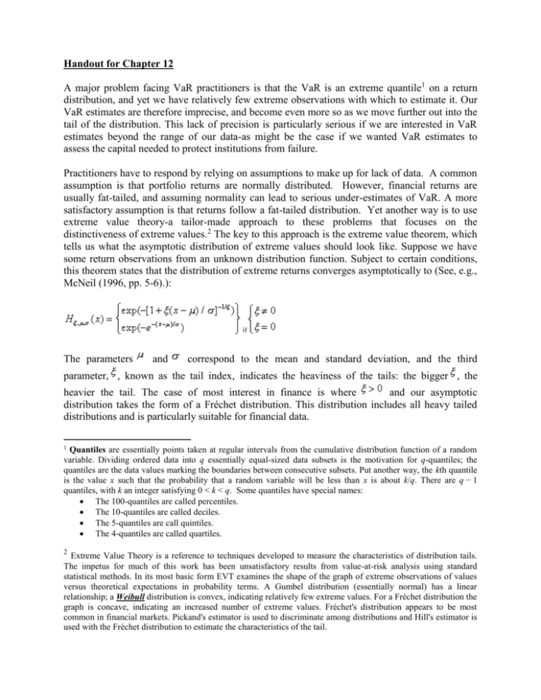
Handout for Chapter 12
A major problem facing VaR practitioners is that the VaR is an extreme quantile1 on a return
distribution, and yet we have relatively few extreme observations with which to estimate it. Our
VaR estimates are therefore imprecise, and become even more so as we move further out into the
tail of the distribution. This lack of precision is particularly serious if we are interested in VaR
estimates beyond the range of our data-as might be the case if we wanted VaR estimates to
assess the capital needed to protect institutions from failure.
Practitioners have to respond by relying on assumptions to make up for lack of data. A common
assumption is that portfolio returns are normally distributed. However, financial returns are
usually fat-tailed, and assuming normality can lead to serious under-estimates of VaR. A more
satisfactory assumption is that returns follow a fat-tailed distribution. Yet another way is to use
extreme value theory-a tailor-made approach to these problems that focuses on the
distinctiveness of extreme values.2 The key to this approach is the extreme value theorem, which
tells us what the asymptotic distribution of extreme values should look like. Suppose we have
some return observations from an unknown distribution function. Subject to certain conditions,
this theorem states that the distribution of extreme returns converges asymptotically to (See, e.g.,
McNeil (1996, pp. 5-6).):
if
The parameters
and
correspond to the mean and standard deviation, and the third
parameter, , known as the tail index, indicates the heaviness of the tails: the bigger , the
heavier the tail. The case of most interest in finance is where
and our asymptotic
distribution takes the form of a Fréchet distribution. This distribution includes all heavy tailed
distributions and is particularly suitable for financial data.
1
Quantiles are essentially points taken at regular intervals from the cumulative distribution function of a random
variable. Dividing ordered data into q essentially equal-sized data subsets is the motivation for q-quantiles; the
quantiles are the data values marking the boundaries between consecutive subsets. Put another way, the kth quantile
is the value x such that the probability that a random variable will be less than x is about k/q. There are q − 1
quantiles, with k an integer satisfying 0 < k < q. Some quantiles have special names:
 The 100-quantiles are called percentiles.
 The 10-quantiles are called deciles.
 The 5-quantiles are call quintiles.
 The 4-quantiles are called quartiles.
2
Extreme Value Theory is a reference to techniques developed to measure the characteristics of distribution tails.
The impetus for much of this work has been unsatisfactory results from value-at-risk analysis using standard
statistical methods. In its most basic form EVT examines the shape of the graph of extreme observations of values
versus theoretical expectations in probability terms. A Gumbel distribution (essentially normal) has a linear
relationship; a Weibull distribution is convex, indicating relatively few extreme values. For a Fréchet distribution the
graph is concave, indicating an increased number of extreme values. Fréchet's distribution appears to be most
common in financial markets. Pickand's estimator is used to discriminate among distributions and Hill's estimator is
used with the Fréchet distribution to estimate the characteristics of the tail.