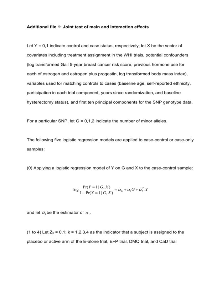
Additional file 1: Joint test of main and interaction effects
Let Y = 0,1 indicate control and case status, respectively; let X be the vector of
covariates including treatment assignment in the WHI trials, potential confounders
(log transformed Gail 5-year breast cancer risk score, previous hormone use for
each of estrogen and estrogen plus progestin, log transformed body mass index),
variables used for matching controls to cases (baseline age, self-reported ethnicity,
participation in each trial component, years since randomization, and baseline
hysterectomy status), and first ten principal components for the SNP genotype data.
For a particular SNP, let G = 0,1,2 indicate the number of minor alleles.
The following five logistic regression models are applied to case-control or case-only
samples:
(0) Applying a logistic regression model of Y on G and X to the case-control sample:
log
Pr(Y  1 | G, X )
  0   1G   2T X
1  Pr(Y  1 | G, X )
and let ̂ 1 be the estimator of  1 .
(1 to 4) Let Zk = 0,1; k = 1,2,3,4 as the indicator that a subject is assigned to the
placebo or active arm of the E-alone trial, E+P trial, DMQ trial, and CaD trial
respectively. Applying a logistic regression model to all the cases in the
corresponding trial component:
log
where log
Pr( Z k  1 | G)
q
 log k   k   k G,
1  Pr( Z k  1 | G)
1  qk
qk
is the offset term, with qk the fraction of women assigned to the
1  qk
active arm in the kth trial component. Denote corresponding parameter estimates to
be ˆ k , ˆk .
A chi-square test with 5 degrees of freedom is used to test the hypothesis that
  1 ,  1 ,  2 ,  3 ,  4 T  0 0 0 0 0T .
Specifically, we reject the null hypothesis if
T
t (ˆ) var(ˆ) 1ˆ   52,0.95 , where ˆ  ˆ1 , ˆ1 , ˆ2 , ˆ3 , ˆ4  ,  52,0.95 is the lower 95th
percentile of chi-square distribution with 5 degrees of freedom, and t(.) denotes
vector transpose.
As shown in [23], ̂ 1 is asymptotically independent of [ˆ1 , ˆ2 , ˆ3 , ˆ4 ], ; thus, the offdiagonal elements in the first row and first column of var(ˆ) will all be zero and
ˆ1 
ˆ 
2
t (ˆ)V (ˆ) 1ˆ  ˆ 1 / var(ˆ 1 )  [ˆ1 , ˆ 2 , ˆ3 , ˆ 4 ] var[ ˆ1 , ˆ 2 , ˆ3 , ˆ 4 ] 1  2  .
ˆ3 
 
ˆ 4 
Note that var(ˆ ) can be obtained from the logistic model fitting in (0), and we
estimate var[ˆ1 , ˆ2 , ˆ3 , ˆ4 ] using a sandwich type estimator.
For subject i in the case-control sample, let U1i, U2i, U3i, U4i be the score function for
 Z ki  E ( Z k | Gi ) 
models 1 to 4, respectively; U ki  
, k  1,2,3,4 if subject i is a case
Gi ( Z ki  E ( Z k | Gi )) 
in trial component k, otherwise Uki = (0,0)T.
Let I1, I2, I3, I4 be the information matrix for models 1 to 4, respectively, with
dimensions of 4x4 each, and let N be the total sample size of the case-control
sample:
I k  i 1 I ki
N
where
Gi E ( Z k | Gi )(1  E ( Z k | Gi )) 
 E ( Z k | Gi )(1  E ( Z k | Gi ))
I ki  

2
Gi E ( Z k | Gi )(1  E ( Z k | Gi )) Gi E ( Z k | Gi )(1  E ( Z k | Gi )) 
if subject i is a case in trial component k, otherwise:
0 0 
I ki  
.
0 0 
Then the sandwich estimator for variance of [ˆ1 , ˆ1 , ˆ2 , ˆ2 , ˆ3 , ˆ3 , ˆ4 , ˆ4 ]T can be
computed as:
 I1
0

0

0
0
0
I2
0
0
I3
0
0
0
0 
0

I4 
1
U 1i 
N U 
 2i U

1i
i 1 U 3i 
 
U 4i 
U 2i
U 3i
 I1
0
U 4i 
0

0
0
0
I2
0
0
I3
0
0
0
0 
0

I4 
1
from which we can obtain estimate of var[ˆ1 , ˆ2 , ˆ3 , ˆ4 ] .
Furthermore, note that since subjects in the E-alone trial and the E+P trial are nonoverlapping, we have ˆ1  ˆ2 , and the covariance term between ˆ1 and ˆ 2 in the
estimate of var[ˆ1 , ˆ2 , ˆ3 , ˆ4 ] is set equal to zero.