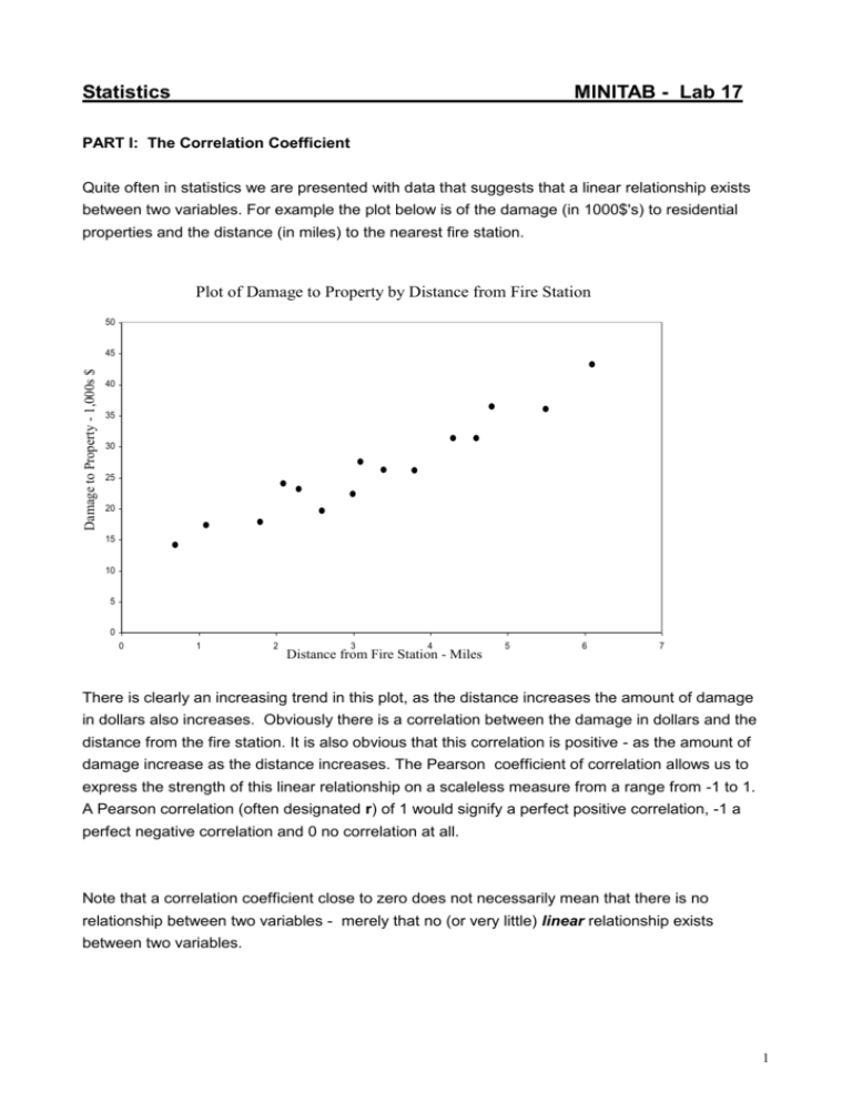
Statistics
MINITAB - Lab 17
PART I: The Correlation Coefficient
Quite often in statistics we are presented with data that suggests that a linear relationship exists
between two variables. For example the plot below is of the damage (in 1000$'s) to residential
properties and the distance (in miles) to the nearest fire station.
Plot of Damage to Property by Distance from Fire Station
50
Damage to Property - 1,000s $
45
40
35
30
25
20
15
10
5
0
0
1
2
3
4
Distance from Fire Station - Miles
5
6
7
There is clearly an increasing trend in this plot, as the distance increases the amount of damage
in dollars also increases. Obviously there is a correlation between the damage in dollars and the
distance from the fire station. It is also obvious that this correlation is positive - as the amount of
damage increase as the distance increases. The Pearson coefficient of correlation allows us to
express the strength of this linear relationship on a scaleless measure from a range from -1 to 1.
A Pearson correlation (often designated r) of 1 would signify a perfect positive correlation, -1 a
perfect negative correlation and 0 no correlation at all.
Note that a correlation coefficient close to zero does not necessarily mean that there is no
relationship between two variables - merely that no (or very little) linear relationship exists
between two variables.
1
Summary from Lecture Notes
The Pearson product movement coefficient of correlation, r, is a measure of the strength of the linear
relationship between two variables x and y. It is computed (for a sample of n measurements on x and y) as
follows:
SS xy
r
Where
SS xy   xi yi 
SS xx   xi2 
SS xx SS yy
 x  y 
i
 x 
i
n
2
i
n
 y 
 y 
n
2
SS yy
2
i
i
The data shown in the plot above is available on the class library as firedamage.MTW. Open this
data set and get the correlation coefficient.
Go to Stat > Basic Statistics > Correlation... and select 'Distance' and 'Damage - $s' as the
two variables, then click OK.
What is the correlation coefficient ? ______________________
In statistics were are interested is using a sample correlation coefficient to estimate the population
correlation coefficient. This involves getting a standard error for the correlation coefficient estimate
and perhaps conducting tests of hypotheses. However as the correlation coefficient is essentially
part of simple linear regression we will do this in Part II of this lab.
PART II:
1.
Simple Linear Regression
In simple linear regression we attempt to model a linear relationship between two variables with a
straight line and make statistical inferences concerning that linear model. We are assuming here
that the variable on the x axis (the distance from the fire station) will predict the amount of fire
damage caused to the house. In this case therefore, distance from the fire station is the predictor
variable and the damage to the property is the response variable.
2
2.
Fitting the Line
Still using the dataset 'firedamage.mtw', create a plot the data .Go to Graph > Plot... and select
'Damage - $' as the y variable and 'Distance' as the x variable, click OK.
When fitting a straight line model we fit what is called the least squares line. This is a straight
line such that the vertical distance between the points and the line is kept at a minimum.
An equation for a straight line model has two components, the intercept and the slope.
Therefore the equation of the least squares line takes the form,
Intercept + slope(predictor variable) +  (the error or residual term)
or more generally:
 0 +  1(predictor variable) + , where  0 is the intercept and  1 is the slope of the line.
 is the distance between the fitted line and the data point, and it is the square of this quantity that
we minimise using the method of least squares.
Summary From Lecture Notes
The formulae for the estimates of the slope and the intercept are;
SS xy
Slope:
̂ 1 
Where
SS xy 
 x  x  y
SS xx 
 x
ˆ 0  y  ˆ1 x
Intercept:
SS x
i
i
 y 
x y
i
i

 x  y 
i
i
n
 x 
 
n
2
n
3.
i
 x
2
xi2
i
= sample size
Statistical Inference
The fitting of the least squares line is essentially mathematical and of itself does not have any
stocastic (i.e. statistical) content. However from a statistical point of view the fitting of the least
squares line is a statistical modelling exercise. We are attempting to estimate the true linear
relationship (i.e. in the population) from sample data. It is possible therefore that the apparent
linear trend seen in the plot is a result of sampling variation and does not reflect an actual linear
relationship between the two variables in the population. Therefore we must conduct an
hypothesis test to compare the amount of variation in the data explained by the linear model with
3
an estimate of background or sampling variation. The approach taken is broadly similar to that of
ANOVA and indeed an ANOVA table is constructed for this purpose.
The Hypothesis being tested in this ANOVA is (in the case of simple linear regression) that the
slope of the line = 0, versus an alternative that the slope of the line is not = 0.
Ho:  1 = 0
Ha:  1  0
And is distributed as F with 1, and n-2 degrees of freedom.
4.
Fitting A Regression Model in MINITAB
Go to Stat > Regression > Fitted Line Plot...
1. Select the response
variable here
2. Select the predictor
variable here
3. Ensure that the
linear model is selcted
This command will given you a plot of the response versus the predictor with the least squares
line shown on the plot, the least squares regression equation will be displayed over the plot as
well as s. If you look at the session window you will also see the ANOVA table for this model and
the associated p value.
What is the least squares regression equation ? ___________________________________
Is the relationship between distance and damage positive or negative ? ________________
Summarise the hypothesis that is being tested in the ANOVA table, include the Ho, Ha, set  =
.01, the test statistic, the p value and state your conclusion.
4
5.
Standard Error of the Slope
We can calculate a standard error of the slope using the s which is our estimate of . This will
allow us to test hypotheses about the slope (more general test than that contained within the
ANOVA table) and also allow us to get a confidence interval for the slope.
Summary from Lecture Notes
The standard error of the slope is
 ˆ 
1

SS xx
which is estimated as s ̂ 
1
s
SS xx
A hypothesis test for the slope
One-Tailed test
Two-Tailed test
Ho: 1 = 10
Ha: 1 < 10 (or 1 > 10)
Ho:  1 = 10
Ha:  1  10
Test statistic: t 
ˆ1   10
s ˆ

ˆ1   10
s
1
SS xx
Rejection Region:
One-Tailed test
Two-tailed test
t < -t
(or t < t )
| t | > t/2
where t and t/2 are based on (n-2) degrees of freedom.
Assumptions: Same assumptions as in previous summary box.
Go to Stat > Regression > Regression...
1. Select the response variable
2. Select the predictor variable
5
What is the standard error of the slope ? __________________________
MINITAB by default tests the two-tailed null hypothesis that the slope is zero. Report the results of
this hypothesis test in the usual way (use  = .01).
Calculate the square root of the F test statistic from the ANOVA table.
What is the result ? ______________
What do notice when you compare this value to the value of the t test statistic for testing the slope
is zero ? __________________________________
6
The Coefficient of Determination - R2
How much of the total sample variability around y is explained by the linear relationship between x
and y ? The answer to this is given by the Coefficient of Determination or R2. The Coefficient of
determination is the ratio between the total variation in the data and variation 'explained' by the
linear relationship between the predictor and response variables.
Coefficient of Determination - R2
R2 =
SS regression / SS Total
What is R2 for the regression model fitted above ? _____________________
Note, that in the case of a simple linear regression model the coefficient of determination is the
correlation coefficient squared. Calculate the square root of R2 and compare it to the correlation
coefficient computed in part I.
6
7
Confidence Interval for the Slope
A confidence interval for the slope may be obtained by using the estimated standard error of the
slope and an appropriate quantile from the t distribution with n-2 degrees of freedom.
Summary From Lecture Notes
ˆ1  t / 2 S ˆ
1
where the estimated standard error of ̂ 1 is calculated by
S ̂ 
1
s
SS xx
and t/2 is based on (n-2) degrees of freedom.
Assumptions:
Where  is defined as
 yi  yˆ i  ,
1. The mean of the probability distribution of  is 0.
2. The variance of the probability distribution of  is equal at all
values of the predictor variable x.
3. The probability distribution of  is normal.
4. The values of  associated with any tow values of y are independent.
Using the standard error from part 5, and either the INVCDF command or the Cambridge tables to
get the appropriate quantile form the t distribution to calculate the 99% confidence interval for the
slope:
What is the confidence interval? (________________ to ________________)
REVISION SUMMARY
After this lab you should be able to :
-
Calculate the correlation coefficient by hand and in Minitab
-
Fit a simple linear regression line to data using Minitab
-
Understand the hypothesis in the simple linear regression ANOVA table
-
Test if the slope of the model is equal to zero or not
-
Construct a confidence interval for the slope
7