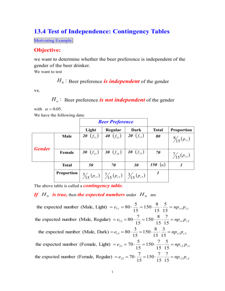
13.4 Test of Independence: Contingency Tables
Motivating Example:
Objective:
we want to determine whether the beer preference is independent of the
gender of the beer drinker.
We want to test
H 0 : Beer preference is independent of the gender
vs.
H a : Beer preference is not independent of the gender
with   0.05 .
We have the following data:
Beer Preference
Male
Gender
Female
Light
20  f11 
5
15
 pc1 
 f 22 
30
50
Total
Proportion
 f 21 
30
Regular
40  f12 
Dark
20  f13 
10
70
7
15
 pc 2 
 f 23 
30
Total
80
70
150 n 
3 p 
15 c 3
Proportion
15
 p r1 
15
 pr 2 
8
7
1
1
The above table is called a contingency table.
If H 0 is true, then the expected numbers under H 0 are
5
8 5
 150  
 np r1 p c1
15
15 15
7
8 7
the expected number (Male, Regular)  e12  80   150    npr1 pc 2
15
15 15
3
8 3
the expected number (Male, Dark)  e13  80   150    npr1 pc 3
15
15 15
5
7 5
the expected number (Female, Light)  e21  70   150    npr 2 pc1
15
15 15
7
7 7
the expected number (Female, Regular)  e22  70   150    npr 2 pc 2
15
15 15
the expected number (Male, Light)  e11  80 
1
the expected number (Female, Dark)  e23  70 
3
7 3
 150    np r 2 pc 3 .
15
15 15
The expected numbers under H 0 can be summarized by
Beer Preference
Male
Gender
Female
Proportion
Light
n  p r1  pc1
Regular
n  p r1  p c 2
Dark
n  p r1  p c 3
 e11  26.67
 e12  37.33
 e13  16
n  p r 2  pc1
n  p r 2  pc 2
n  p r 2  pc 3
 e21  23.33
 e22  32.67
 e23  14
5
15
 pc1 
7
15
 pc 2 
eij , i  1, 2; j  1, 2, 3 ,
15
 p r1 
15
 pr 2 
8
7
3 p 
15 c 3
f ij
Intuitively, if the differences between the observed number
number (under H 0 )
Proportion
and the expect
are small, that might imply
H 0 is true and thus the observed number and the expected number (under H 0 )
are close. The following statistic can be used to reflect the difference between the
observed number and the expected number,
2
3
  
2
i 1 j 1
f
 eij 
2
ij
eij


 f11  e11 2  f12  e12 2  f13  e13 2

e11

e12
e13
 f 21  e21 2  f 22  e22 2  f 23  e23 2
e21

e22

e23
2
2
2

20  26.67  40  37.33 20  16



26.67
37.33
16
2
2
2

30  23.33 30  32.67  10  14



23.33
32.67
14
 6.13
2
General Case:
Suppose there are two variables, column variable (with m categories)
and row variable (with p categories). We want test the hypothesis
H 0 : Row variable is independent of column variable
vs.
H a : Row variable is not independent of column variable.
Suppose the sample size is n. The contingency table is
Column Variable (m columns)
1
1
Row
Variable
(p rows)
f11


i
f i1

p
f p1
p
k 1
f1 j

…
…
…

f pj
pcj 

k 1
n
…
…
…
proportions
f1m
m
p r1 

p ri 

n
p rp 
km
n
If H 0 is true, then the expected numbers under H 0 are
3
n
f
k 1
ik
n
m
pcm 
k 1
1k

f pm
f
k 1
m
p
f kj
f

f im

p
f k1
…
m

f ij

p c1 

…
…
j


proporti
ons
...
f
k 1
n
1
pk
Column Variable (m columns)
1
1
e11 
...
…
npr1 pc1
Row
Variable
(p rows)
j
e1 j 
…
m
proportions
…
e1m 
p r1
np r1 pcm
np r1 pcj






i
ei1 
…
eij 
…
eim 
np ri pc1


p
e p1 
…
np rp pc1
proporti
ons
p c1
np ri p cm
np ri pcj


e pj 



…
eim 
p rp
nprp pcm
nprp pcj
…

p ri
…
p cj
p cm
1
Note:
eij  np ri p cj  sample size   row i proportion   colmmn j proportion 

  p
   f kj 
   k 1   sample size    row i total
 sample size
  n 


 
 


  p
f ik     f kj 
  k 1  row i total   column j total 

n
sample size
 m
  f ik
 n   k 1
 n



 m

 k 1
  column j total 
  

  sample size 
where
m
p
k 1
k 1
row i total   f ik , column j total   f kj , i  1,, p; j  1,, m.
and
4
p
m
sample size   f ij  n .
i 1 j 1
Thus, the chi-square statistic used to reflect the difference between the
observed number and the expected number is
p m
  
2
f
 eij 
2
ij
i 1 j 1
eij
2
2
2

f1m  e1m 

f11  e11   f12  e12 



e11
e12
e1m
2
2
2

f 2 m  e2 m 

f 21  e21   f 22  e22 



e21
f

 e p1 
2
p1
e p1
Next question: how large
e22
f

2
 ep2 
2
p2
ep2
e2 m
f

 e pm 
2
pm
e pm
must be to reject H 0 ?
Chi-Square Test:
Let
p
m
 2  
f
i 1 j 1
As
 eij 
2
ij
eij
eij  5 for every i and j, the chi-square test with level of
significance

for
H 0 : Row variable is independent of column vairalbe
vs.
H a : Row variable is not independent of column variable.
is to
5
where
reject H 0 :
 2   2p 1m 1,
not reject H 0 :
 2   2p 1m 1,
 2p1m1,
,
can be obtained by


P  2p 1m 1   2p 1m1,   .
In addition,

p - value  P 
2
 p 1m1

2

.
Note: as H 0 is true, the random variable with sample value
2
is
 2p1m1 .
Example (continue)
Since
p  2, m  3
we reject
and
 2  6.13  5.99   22,0.05   2p1m1, ,
thus
H 0 . Also,

 

p  value  P  2p1m1   2  P  22  6.13  0.047  0.05   ,
we also reject
H 0 based on p-value. Therefore, we conclude that the beer
preference is not independent of the gender of the beer drinker.
Example:
The following data are the number of people who are in favor of, are not in favor of,
and have no comment on, some proposal:
Male
Female
Favor
252
148
Not Favor
145
105
No Comment
203
147
Please test if female and male differ in their opinions about the proposal with
  0.05 .
[solution:]
The column totals are 252  148  400,145  105  250,203  147  350
6
while the row totals are 252  145  203  600,148  105  147  400 . In
addition, the total number is 1000.
The table for the expected numbers
eij
is
Favor
Not Favor
No Comment
Row Total
600
Male
600  400
 240
1000
600  250
 150
1000
600  350
 210
1000
Female
400  400
 160
1000
400  250
 100
1000
400  350
 140
1000
400
Column Total
400
250
350
1000
Thus,
p
m
  
2
f
i 1 j 1
 eij 
2
ij
eij
3
2
 
i 1 j 1
f
 eij 
2
ij
eij
2
2
2



252  240 
145  150 
203  210 



240
150
210
2
2
2



148  160 
105  100 
147  140 



 2.5
160
100
140
Since
 2  2.5  5.99   22,0.05  22131,0.05  2p1m1, , we do not
reject
H0 .
Online Exercise:
Exercise 13.4.1
Exercise 13.4.2
7