Understanding the Formulas
for the CFP Certification Examination
By
David W. Durr, Ph.D., CFA, CFP®
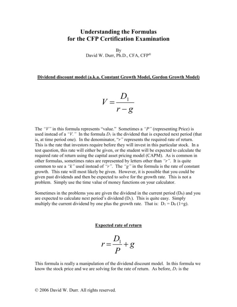
Dividend discount model (a.k.a. Constant Growth Model, Gordon Growth Model)
D1
V
rg
The “V” in this formula represents “value.” Sometimes a “P” (representing Price) is
used instead of a “V.” In the formula D1 is the dividend that is expected next period (that
is, at time period one). In the denominator, “r” represents the required rate of return.
This is the rate that investors require before they will invest in this particular stock. In a
test question, this rate will either be given, or the student will be expected to calculate the
required rate of return using the capital asset pricing model (CAPM). As is common in
other formulas, sometimes rates are represented by letters other than “r”. It is quite
common to see a “k” used instead of “r”. The “g” in the formula is the rate of constant
growth. This rate will most likely be given. However, it is possible that you could be
given past dividends and then be expected to solve for the growth rate. This is not a
problem. Simply use the time value of money functions on your calculator.
Sometimes in the problems you are given the dividend in the current period (D0) and you
are expected to calculate next period’s dividend (D1). This is quite easy. Simply
multiply the current dividend by one plus the growth rate. That is: D1 = D0 (1+g).
Expected rate of return
D1
r g
P
This formula is really a manipulation of the dividend discount model. In this formula we
know the stock price and we are solving for the rate of return. As before, D1 is the
© 2006 David W. Durr. All rights reserved.
dividend that is expected next period. Also, “g” is the constant rate of growth. Notice
that this formula uses “P” to represent stock price.
Remember that dividend divided by price gives us the dividend yield. So, this formula
says that the expected rate of return on this stock is equal to the expected dividend yield
plus a growth factor. This is consistent with what we know about investing in equity
securities. The return to an equity investor will come from either the dividend yield
and/or the growth in the value of the asset (capital appreciation).
Covariance
COVij ij i j
Covariance is a measure of how much two assets move together. It is a measure that
combines the volatility of one stock’s returns with the tendency of those returns to move
up or down at the same time that another stock’s returns move up or down.
The covariance of two assets is calculated by multiplying the standard deviation of one
stock’s returns by the standard deviation of another stock’s returns by the correlation
coefficient (that is, the correlation between the two sets of returns). In this formula, the
correlation coefficient (for assets “i” and “j”) is represented by “ρij “. While this
symbol looks like the letter “p” it is actually the lower case Greek letter “rho.” You
should know that many professors and textbooks substitute an “r” in place of “rho” when
presenting the formula for covariance. In that case, the correlation between assets “i”
and “j” would be denoted as “rij”. The standard deviation symbol is represented by the
lower case Greek letter “sigma.” So, “σi” represents the standard deviation of security “i”
and “σj” represents the standard deviation of security “j.”
Standard deviation of a two-asset portfolio
p Wi 2 i2 W j2 2j 2Wi W j COVij
This is one of the more complicated-looking formulas that you will work with for the
exam. But, remember that the formula is provided so you only need to know which
information to plug into the formula and then understand the concepts and implications.
© 2006 David W. Durr. All rights reserved.
The weights (that is, percentage of your money invested in each asset) must add to 100
percent. Since this is for a two-asset portfolio (asset i and asset j), then Wi is the percent
of money invested in asset i and Wj is the percent of your money invested in asset j.
Remember that standard deviation is denoted by the Greek letter σ. Therefore, the
standard deviation of the portfolio is σp, the standard deviation of asset i is σi and the
standard deviation of asset j is σj. COVij is the covariance of asset i and asset j.
Remember that since the formula for covariance is ρijσiσj then you could substitute this
term into the formula for the portfolio standard deviation and it becomes:
p Wi 2 i2 W j2 2j 2Wi W j ij i j
Beta
i
COVim
m2
im i
m
Beta is a measure of an asset’s systematic risk. There are other similar terms for this type
of risk. In fact, it is also correct to say: beta measures an asset’s nondiversifiable risk;
and beta measures an asset’s market risk.
This formula shows that an asset’s beta can be calculated by dividing the covariance
(between an asset’s return and the market return) by the variance of the market returns
(remember that variance is denoted by σ2, which is the standard deviation squared). This
formula simplifies to:
i
COVim
m2
im i m im i
m m
m
These terms cancel
© 2006 David W. Durr. All rights reserved.
Standard deviation of historical returns (population)
n
r
r r
t 1
2
t
n
This formula is used to determine the population standard deviation of a set of stock
returns. In this equation, the standard deviation of returns is denoted by σr. This formula
directs us to take each return that occurred in a past period (rt) and subtract from that
return the arithmetic average return ( r ). We then square that difference. Next, we add
together all of the squared differences (the Σ in the equation means to “sum”). We divide
this amount by the total number of returns that we used. This gives us the variance of the
population (which, by the way is denoted as σ2). When we take the square root of the
variance we get the standard deviation.
Standard deviation of historical returns (sample)
n
sr
r r
t 1
2
t
n 1
This formula is used to determine the sample standard deviation of a set of stock returns.
In this equation, the standard deviation of the sample is denoted by sr. As you can see,
this formula is very similar to the formula used to calculate the standard deviation of a
population. The only difference is in the denominator. This formula directs us to take
each return that occurred in a past period (rt) and subtract from that return the arithmetic
average return ( r ). We then square that difference. Next, we add together all of the
squared differences. We divide this amount by the total number of returns that we used,
minus one. This gives us the variance of the sample. When we take the square root of
the variance we get the standard deviation.
© 2006 David W. Durr. All rights reserved.
Conversion value of a convertible bond
CV
Par
x Ps
CP
Some bonds contain an option that allows the bond holder to convert the bond into a
fixed number of shares of common stock. This formula is used to determine the
conversion value (CV), should a bond holder elect to exercise the option. The bond
indenture will specify the price at which the shares can be converted. This price is
referred to as the conversion price and is represented by “CP” in the formula. If we
divide the par value of the bond by the conversion price, we are able to determine the
total number of shares (called the conversion ratio) that will be received upon conversion.
When we multiply the number of shares we can receive by the current market price (Ps)
of the firm’s common stock, we get the conversion value.
For example, assume there is a $1,000 par value convertible bond. The conversion price
is specified to be $40. The bond holder therefore has the option to convert the bond into
25 shares (the conversion ratio is $1,000 / $40). If the current market price of the
common stock is $42.50 per share, then the conversion value is equal to $1,062.52
(calculated as follows: 25 shares times $42.40 per share).
Capital asset pricing model (also the security market line)
ri rf (rm rf ) i
This is one of the more important concepts in the investment material. The capital asset
pricing model (CAPM) is used to determine the required rate of return on an asset, given
its level of systematic risk. In this formula, the required rate of return on a risky asset is
equal to the risk free rate (rf) plus a risk premium (represented by ( rm – rf )βi in the
equation) to compensate the investor for taking on market risk. The risk premium for the
particular asset is determined by multiplying the market risk premium (which is ( rm – rf )
in the equation) by the asset’s beta coefficient (βi ).
Now, this is another one of the formulas in which the notations for some of the variables
are sometimes inconsistent. It is common to see the “r” replaced with a “k.” Sometimes
the beta (β) is denoted simply with a “b.” So, the formula could take many forms
including:
© 2006 David W. Durr. All rights reserved.
ki krf (km krf ) bi
The formula for the capital asset pricing model is actually the equation of a line. When
CAPM is graphed, the line is called the security market line (SML). The SML shows the
relationship between an asset’s systematic risk and the required rate of return. Assets
with greater risk are expected to provide higher rates of return. The graph takes the
following form:
SML
Return (Ri)
rm
rf
1.0
Risk (β)
Capital market line
rm rf
rp rf p
m
The formula for the capital market line (CML) is quite similar to the formula for the
security market line (SML). The main differences between the two models are: 1) the
CML is used to express the risk and return relationship for diversified portfolios only,
whereas the SML can be used to show the relationship between risk and return for any
asset; and 2) the CML uses standard deviation as the risk measure, whereas the SML uses
beta.
© 2006 David W. Durr. All rights reserved.
In the formula, the required rate of return for the portfolio (rp) is equal to the risk free rate
of return plus a portfolio risk premium. The risk premium for the portfolio is equal to the
market risk premium (the term in brackets) multiplied by the standard deviation for the
portfolio. Note that the term in brackets is simply the excess market return divided by the
standard deviation for the market. This “excess market return per unit of market risk” is
multiplied by the risk of the portfolio. This determines the risk premium that investors
require before investing in this portfolio. The graph showing the CML is as follows:
CML
Return (Rp)
rm
rf
σp
Risk (standard deviation)
Sharpe ratio
Sp
rp rf
p
The Sharpe ratio is a risk-adjusted measure of portfolio performance. In the formula, the
portfolio return is denoted by rp. The risk free rate is denoted by rf. In the numerator of
the equation you have the excess return. That is, it is the return that the portfolio earned
that is in excess of the risk free rate of return. A portfolio manager certainly hopes that
the numerator is positive. Otherwise, the portfolio (composed of risky assets) earned less
than could have been earned if the funds had been invested in risk free Treasury
© 2006 David W. Durr. All rights reserved.
securities. The excess return is then divided by the standard deviation of the portfolio
(σp). This ratio gives the excess portfolio return per unit of total risk.
You should remember that the Sharpe ratio is a relative measure of performance. This
means that the value of the ratio is difficult to interpret on its own. It must be compared
to another Sharpe ratio. Consider the following example. Assume that ABC Value
Portfolio earned an 11.65 percent return last period. The risk free rate during the same
time period was 5.25 percent. The standard deviation of the portfolio was 12 percent.
The return on the S&P 500 was 12.0 percent and the standard deviation for the S&P 500
was 15.3 percent. The Sharpe ratio for the ABC Value Portfolio (Sp) and the Sharpe ratio
for the S&P 500 (Sm) are computed as follows:
Sp
11.65 5.25
.533
12
Sm
12.0 5.25
.44
15.3
We can conclude that the ABC Value Portfolio outperformed the market (S&P 500) on a
risk-adjusted basis.
Alpha (Jensen’s Alpha)
p rp [rf (rm rf ) p ]
Jensen’s alpha is an absolute measure of performance. In essence, the value of alpha
indicates the value added to (or subtracted from) the portfolio as a result of portfolio
management. Alpha is denoted by the Greek letter alpha (α) although sometimes you see
it simply as a lowercase “a”. The formula shows that the alpha of the portfolio αp is
equal to the actual portfolio return “rp” minus the following term: [rf + (rm – rf)βp].
You should recognize the term in brackets: it is the capital asset pricing model that is
used to produce the required rate of return for an asset. So, the alpha of the portfolio is
simply the actual portfolio return minus the return that the investor expected to earn when
they invested in the asset.
Consider the previous example. Assume that ABC Value Portfolio earned an 11.65
percent return last period. The risk free rate during the same time period was 5.25
percent. ABC Value Portfolio has a beta of .80. The return on the S&P 500 was 12.0
percent. The alpha for the ABC Value Portfolio is computed as follows:
© 2006 David W. Durr. All rights reserved.
p 11.65 [5.25 (12.0 5.25) .80] 1.0
We can conclude that the ABC Value Portfolio outperformed expectations by one percent
on a risk-adjusted basis.
Treynor Ratio
Tp
rp rf
p
The Treynor ratio is also a risk-adjusted measure of portfolio performance. As with the
Sharpe ratio, the portfolio return is denoted by rp and the risk free rate is denoted by rf.
The excess portfolio return is again expressed in the numerator of the equation
(remember this is the return that the portfolio earned that is in excess of the risk free rate
of return). The excess return is then divided by the beta of the portfolio (βp). This ratio
gives the excess portfolio return per unit of systematic risk.
The Treynor ratio (like the Sharpe ratio) is a relative measure of performance. This
means that the value of the Treynor ratio is difficult to interpret on its own. It must be
compared to another Treynor ratio to assess performance. Consider the previous
example. Assume that ABC Value Portfolio earned an 11.65 percent return last period.
The risk free rate during the same time period was 5.25 percent. ABC Value Portfolio
has a beta of .80. The return on the S&P 500 was 12.0 percent. The Treynor ratios for
the ABC Value Portfolio and for the S&P 500 are computed as follows:
p
11.65 5.25
8 .0
.8
m
12.0 5.25
6.75
1.0
We know that both the Treynor ratio and the Jensen measure (alpha) use beta to assess
risk. Remember that beta is one of the statistics produced in a statistical regression (when
portfolio returns are regressed against market returns). Another important statistic from
the same regression is r2 (the coefficient of determination). In a way, the coefficient of
determination tells us how “good” our regression is. If the regression produces a high
value of r2 then this means that the regression is “good” and the statistics it produced
(including beta) are “good.” If the regression produces a low value of r2 then the
© 2006 David W. Durr. All rights reserved.
regression is “not good” and the resulting statistics (including beta) are not reliable. In
this case, you should not use Treynor or Jensen (alpha) to evaluate portfolio performance
because both of these measures use beta to assess portfolio risk. In this case, you should
use the Sharpe ratio to evaluate portfolio performance. Since Sharpe uses standard
deviation, it is not influenced by the regression statistics.
Bond Duration
n
ct (t )
t
(
1
i
)
D t n1
ct
t
t 1 (1 i )
There are two advantages of this formula. One, it highlights the fact that duration is, by
definition, a time weighted payback. The denominator of the formula is the bond price.
The numerator of the formula includes each future cash flow multiplied by the year in
which it occurs. So, the formula shows us that the duration of a bond is a time-weighted
payback with the each future cash flow weighted by the year in which it occurs.
Ct is the cash flow that occurs in period t. The total number of periods is denoted by n.
The yield to maturity for this bond is denoted by i.
However, the real value of this formula is that it helps us appreciate the next formula,
which is much, much more simple and the recommended approach to solve for bond
duration. I do not believe that you should use this formula to solve for bond duration,
under any circumstance.
Bond Duration
D
1 y (1 y ) t (c y )
y
c [(1 y )t 1] y
While this is a scary looking formula, it is really not that bad. Keep in mind that it will
be provided on the CFP exam, so don’t try to memorize it. Just be able to plug in the
appropriate variables, and then carefully perform the mathematics.
© 2006 David W. Durr. All rights reserved.
The three variables represented in this formula are:
C = coupon rate
Y = yield to maturity
T = time to maturity
Coupon rate will be entered as a decimal. For a bond with a 6 percent coupon rate, you
will enter .06 in the formula. Yield will also be entered as a decimal. If this bond is
currently priced to yield 6.5 percent, you will enter .065 in the formula. Time to maturity
is entered as a whole number. If there are 13 years remaining until the bond matures,
then you will enter 13 in the formula.
For example:
D
1.065 (1.065) 13(.06 .065)
9.29
.065
.06 [(1.065)13 1] .065
Estimating a price change (using duration)
y
P
D
P
1 y
In this formula, “P” represents “price.” The Greek letter delta (Δ) means “change.”
Therefore, ΔP means the change in price. If you divide ΔP by price, this gives you the
percentage price change. As we know, the price of a bond changes in response to
changes in interest rates. We also know that bond duration is a measure of a bond’s price
sensitivity to interest rate changes. This formula can be used to estimate the percentage
that a bond’s price will change when interest rates change.
In the formula, D is the bond’s duration. The market interest rate, or yield, is denoted by
“y.” In the numerator of the ratio we have Δy which is the change in yield. The
denominator is simply one plus the yield (1+y).
Assume that a bond has a duration equal to 8 years. Further assume that the market rate
of interest is 5 percent (0.05). If the interest rate increases to 6 percent (0.06) then the
change in market yield (Δy) is 0.01. The change in yield is calculated by subtracting the
old rate from the new rate (.06 - .05 = .01). The estimated percentage price change is:
© 2006 David W. Durr. All rights reserved.
P
.01
8
.076
P
1
.
05
We expect the value of the bond to fall by 7.6 percent.
Consider another example in which the interest rate falls. Assume a bond has a duration
equal to 7.5 years. The market interest rate falls from 5 percent to 4.5 percent. In this
example, then the change in market yield (Δy) is -0.005. The change in yield is
calculated by subtracting the old rate from the new rate (.045 - .05 = -.005). The
estimated percentage price change is:
P
.005
7.5
.0357
P
1.05
We expect the value of the bond to increase by 3.57 percent.
© 2006 David W. Durr. All rights reserved.


