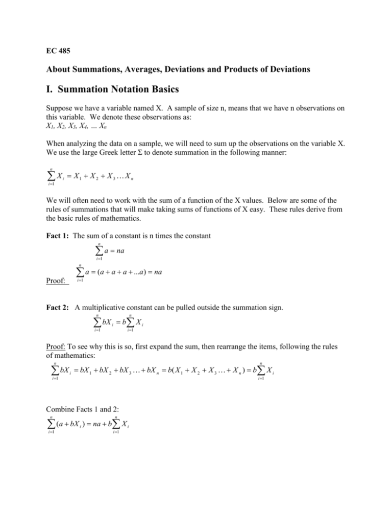
EC 485
About Summations, Averages, Deviations and Products of Deviations
I. Summation Notation Basics
Suppose we have a variable named X. A sample of size n, means that we have n observations on
this variable. We denote these observations as:
X1, X2, X3, X4, … Xn
When analyzing the data on a sample, we will need to sum up the observations on the variable X.
We use the large Greek letter Σ to denote summation in the following manner:
n
X
i 1
i
 X1  X 2  X 3  X n
We will often need to work with the sum of a function of the X values. Below are some of the
rules of summations that will make taking sums of functions of X easy. These rules derive from
the basic rules of mathematics.
Fact 1: The sum of a constant is n times the constant
n
 a  na
i 1
n
 a  (a  a  a  ...a)  na
i 1
Proof:
Fact 2: A multiplicative constant can be pulled outside the summation sign.
n
n
i 1
i 1
 bX i  b X i
Proof: To see why this is so, first expand the sum, then rearrange the items, following the rules
of mathematics:
n
 bX
i 1
n
i
 bX 1  bX 2  bX 3   bX n  b( X 1  X 2  X 3   X n )  b X i
i 1
Combine Facts 1 and 2:
n
 (a  bX
i 1
n
i
)  na  b X i
i 1
Proof: Notice how we can push the summation sign through terms that are joined by summation,
then aplly facts 1 and 2:
n
 (a  bX
i
i 1
n
n
n
i 1
i 1
i 1
)   a   bX i  na  b X i
II. Statistcs and the Use of Summations
Define the sample average as:
n
 Xi
i 1
X 
Define :
n
Thus, you should be able to prove that
n
Fact 1:
(X
i 1
i
 X)  0
once you recognize that the sample average X acts like a constant in much the same way as a is
a constant in the first equation because neither has an i subscript.
Here are a few facts about working with products of deviations from means. You should be able
to prove them:
Fact 2:
n
n
i 1
i 1
 ( X i  X )(Yi  Y )   ( X i  X )Yi
For the same reason, the following is true:
Fact 3:
n
n
i 1
i 1
 ( X i  X ) 2   ( X i  X )X i
The following fact is useful when deriving the Least Squares formula as the solution to the
problem of minimizing the sum of squared residuals with respect to the slope estimate:
Show that:
n
n
n
n
 X i  Yi
i 1
n
 ( X i  X )(Yi  Y )   ( X iYi )  i1
Fact 4:
i 1
i 1
Also, sometimes it is useful to express the formula for the slope estimate in a way that clearly
shows it to be linear function in the Yi data.
n
n
 ( X i  X )(Yi  Y )  ( X i  X )Yi
i 1
Fact 5: ̂1 

n
 ( X i  X )2
i 1
n
 ( X i  X )2
i 1
n
  ai Yi
i 1
i 1
where
ai 
(Xi  X )
n
(Xi  X )
.
2
i 1
A few facts about this ai term (which, by the way, has nothing to do with the a in the a + bX
expression at the top of this document). First recognize that the denominator of the term is the
sum of squared deviations of X from its mean. This sum is some fixed quantity. It functions as a
constant in much the same way as the sample average acted as a constant Result 3 above.
Therefore, when we sum up the values of ai, we can pull the denominator out, and use Result 3
from above.
n
Fact A1:
 ai  0
i 1
Proof:
n
i 1
(Xi  X )
n
 ai  
i 1
n
(Xi  X )

n
1
n
(Xi  X )
2
i 1
(Xi  X ) 
2 i 1
i 1
1
n
(Xi  X )
0  0
2
i 1
n
Fact A2:
 ai X i  1
i 1
Proof:
n
n
n
 ai X i  
i 1
i 1
(Xi  X )Xi
n
(Xi  X )
i 1
2

1
n
 ( X i  X )2
 ( X i  X )X i  in1
 ( X i  X ) 2 i1
 ( X i  X )2
n
i 1
i 1
1
n
Fact A3:
a
i 1
2
i

1
n
(X
i 1
i
 X )2
Proof:
2


n
n 
(Xi  X ) 
1
2

 
a



i
n
2
2 
i 1
i 1 
n
2
(
X

X
)
i
 

 ( X i  X ) 
i 1
 i 1

n
(X
i 1
i
 X )2 
1
n
(X
i 1
i
 X )2
Random Variables, Expected Values of Random Variables and Variances of
Random Variables.
All random variables are assumed to have a probability distribution that tells us the possible
values for the random variable and the associated probabilities of these values. This information
can be used to compute the expected value of the random variable (also known as the mean of
the distribution). This expected value is a weight average of the possible values using
probabilities for weights (below we assume that the random variable x can take on k different
values). Therefore, assume that we have a random variable Xi
k
E ( X )   x   xi p i
i i
k
 2  Var ( X )   ( xi   x ) 2 pi
i i
Suppose we have a new random variable Z that is a function of the underlying random variable
X. The mean and variance of the new random variable can be determined from the mean and
variance of the underlying random variable X and information about how Z is created from X:
Z  a  bX
E ( Z )  E (a  bX )  a  bE ( X )  a  b x
Var ( Z )  Var (a  bX )  b 2Var ( X )  b 2 2
How does this apply to Least Squares?
Well, our estimators ̂ o and ̂ 1 are functions of the sample data on X and Y. Remember that the
data on Y are random. It is generated by the data generating process: Yi   o  1 X i  ui . Note
that the randomness in Y comes from the error term. The parameters  o and 1 are not random,
but instead are unknown parameters. When we examine the formula for ̂ 1 we see that it is a
function of the Y variable, which itself is random due to the underlying error term:
n
n
i 1
i 1
ˆ1   ai Yi   ai (  o  1 X i  u i )
Therefore, ̂ 1 is a random variable. We want to know the expected value ( a.k.a. mean) and
variance of ̂ 1 . The expected value for ̂ 1 is just the expected value of the above expression:
n
 n
 n
E ( ˆ1 )  E   ai Yi    ai E (Yi )   ai E (  o  1 X i  u i )
i 1
 i 1
 i 1
The variable Y is random, but the variable ai is not. For the last term on the right, the only
random element inside the E(.) function is the error term, u. We can pass the E(.) operator
through, using the rules of expectation from above.
n
n
i 1
i 1
E ( ˆ1 )   ai E (  o  1 X i  u i )   ai (  o  1 X i  E (u i ))
Now we need to use the assumption that E(u) = 0 and the Rules about the ai values from above to
prove that the slope estimator is unbiased:
n
E ( ˆ1 )   ai (  o  1 X i  E (u i ))
i 1
n
n
n
n
n
i 1
i 1
i 1
i 1
i 1
  ai (  o  1 X i )   ai  o   ai 1 X i   o  ai  1  ai X i   o (0)  1 (1)  1
For the variance of the slope estimator, we need to make use of several assumptions, such as the
error term is serially uncorrelated and homoskedastic. Also, the data on X are nonrandom and
thus drop out of the variance expression. As before, the only item that is random, and thus
subject to random variation is the error term, u.
 n
 n
 2ˆ1  Var ( ˆ1 )  Var  ai Yi    ai2Var (Yi )
 i 1
 i 1
n
n
n
  a Var (  o  1 X i  u i )   a Var (u i )   a   
i 1
2
i
i 1
2
i
i 1
2
i
2
u
n
2
u
a
i 1
2
i

 u2
 X
n
i 1
n
The last step uses the fact that
 ai2 
i 1
1
n
 X i  X 
i 1
2
 X
2
i
. This is Rule 3 about the ai values.