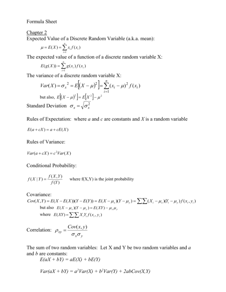
Formula Sheet
Chapter 2
Expected Value of a Discrete Random Variable (a.k.a. mean):
n
  E ( X )   xi f ( xi )
i 1
The expected value of a function of a discrete random variable X:
n
E ( g ( X ))   g ( xi ) f ( xi )
i 1
The variance of a discrete random variable X:


n
Var( X )   x  E  X      ( xi   ) 2 f ( xi )
2

   
but also, E  X     E X
2
2
2
i 1
2
Standard Deviation  x   x2
Rules of Expectation: where a and c are constants and X is a random variable
E (a  cX )  a  cE ( X )
Rules of Variance:
Var (a  cX )  c 2Var ( X )
Conditional Probability:
f (X | Y) 
f ( X ,Y )
f (Y )
where f(X,Y) is the joint probability
Covariance:
Cov( X , Y )  E( X  E( X ))(Y  E(Y ))  E( X   x )(Y   y )   ( X i   x )(Yi   y ) f ( xi , yi )
but also E ( X   x )(Y   y )  E ( XY )   x  y
where E( XY )   X i Yi f ( xi , yi )
Correlation:  xy 
Cov( x, y )
 x y
The sum of two random variables: Let X and Y be two random variables and a
and b are constants:
E(aX + bY) = aE(X) + bE(Y)
Var(aX + bY) = a2Var(X) + b2Var(Y) + 2abCov(X,Y)
Sample Statistics: assume a sample of T observation on Xt
T
Sample Mean
Sample Variance
Sample Standard Deviation
Sample Covariance
Sample Correlation
X
sx2
 Xt
t 1
T
( xi  x )2


T 1
sx  sx2
S xy 
r
1
( xt  x )( yt  y )

T 1
S xy
sx2 s 2y

 ( xt  x )( yt  y )
 ( xt  x )2  ( yt  y )2
Chapter 3 and 4 Formulas
The Method of Least Squares
Yt  1   2 X t  et , the Least Squares estimator is
For the linear model :
comprised of the following 2 formulas (where T is the size of the sample):
b1  Y  b2 X
b2 
T  X t Yt   X t  Yt
T  X t2   X t 
2
Note that b2 could also be calculated using one of the other 3 formulas:
b2 
 X t  X Yt  Y 
2
 X t  X 
b2 
 X t  X Yt
2
 X t  X 
b2   wt Yt
where wt 
X t  X 
2
 X t  X 
These estimators have the following means and variances:
E (b1 )  1 and E (b2 )   2
Var(b1 ) 
 2  X t2
and Var(b2 ) 
T  X t  X 
2
2
 X t  X 
2
se(b1 )  Var(
where 2 is the variance of the error term and is assumed constant.
The estimated line is: Yˆt  b1  b2 X t and a residual is eˆt  Yt  Yˆt
The estimator of  is ˆ
2
2
eˆt2


T 2
so that
se(b1 )  Vaˆr (b1 ) and se(b2 )  Vaˆr (b2 ) where a “hat” means that ˆ 2 has been used in
place of 2 in the variance formulas.
Chapter 5 and 6 Equations
From Section 5.3: The Least squares predictor uses the estimated model to make a
prediction at xo.
yˆ o  b1  b2 xo
The estimated variance of the prediction error is:
 1
( xo  x )2 
vâr( f )  ˆ 1  
 T
 ( xt  x )2 

R-squared is:
2
R2 
SSR
SSE
1
SST
SST
where
SST   ( yt  y ) 2
SSE   eˆt2
So that
R 1
2
 eˆt2
 ( yt  y ) 2
Chapter 7 and 8
For the multiple regression model:
ˆ 2
Vaˆr (b2 ) 
Vaˆr (b3 ) 
(1 
2
r23
)
 ( x 2t  x 2 )
ˆ
yt  1   2 x2t   3 x3t  et
2

2
eˆt2


T k
2
2
(1  r23
) ( x3t  x3 ) 2
Adjusted R-squared:
F-statistic:
F
R 1
2
 eˆt2 /(T  k )
 ( yt  y )2 /(T  1)
( SSER  SSEU ) / J
SSEU /(T  k )
Let SSER be the sum of squared residuals from the Restricted Model
Let SSEU be the sum of squared residuals from the Unrestricted Model.
Let J be the number of “restrictions” that are placed on the Unrestricted
model in constructing the Restricted model. Let T be the number of observations
in the data set. Let k be the number of RHS variables plus one for intercept in the
Unrestricted model.
Chapter 11
Goldfeld Quandt statistic:
ˆ12 SSE1 /(t1  k )
GQ  2 
ˆ 2 SSE2 /(t2  k )
This statistic has an F distribution with t1-k degrees of freedom in the numerator
and t2-k degrees of freedom in the denominator
The variance for b2 when the error term is heteroskedastic is:
Var(b2 )  Var(  2   wt et )
  wt2Var(et )   wt2 t2
(xt  x )2 t2


 ( xt  x )2 2
White standard errors use this Var(b2) formula, using eˆt2 as an estimate for  t2 .
Chapter 12
T
 (eˆt  eˆt 1 ) 2
Durbin-Watson test statistic is calculated as:
d  t 2
T
 eˆt 2
t 1
 2  2 ̂
T
and
̂ 
 eˆ eˆ
t 2
T
t t 1
 eˆ
t 1
2
t