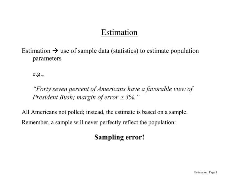
Estimation
Estimation  use of sample data (statistics) to estimate population
parameters
e.g.,
“Forty seven percent of Americans have a favorable view of
President Bush; margin of error  3%.”
All Americans not polled; instead, the estimate is based on a sample.
Remember, a sample will never perfectly reflect the population:
Sampling error!
Estimation: Page 1
Two types of estimates:
(1) Point estimate: single number as the estimate of an unknown quantity
e.g., Answering w/ a single value, what was the outdoor temperature in Oxford right
before class today?
____ degrees
How sure are you of this estimate?
(2) Interval estimate / confidence interval (CI): a range of values as the estimate of an
unknown quantity; when accompanied w/ a specific confidence level or probability,
called confidence intervals
e.g., Answering w/ a range of values, what was the outdoor temperature in Oxford
right before class today?
Between _____ & _____ degrees
How sure are you of this estimate?
**There is a trade-off between precision & confidence**
Estimation: Page 2
Hypothesis Testing vs Estimation
Similar 
Both use sample data to infer something about a population
Different  Designed to answer different questions
Did a new drug lower cholesterol levels?
Measure cholesterol of 25 patients before drug & after
Change in cholesterol is 15 points (225 before; 210 after)
Hypothesis test: Did the drug alter cholesterol levels?
yes/no decision
Reject or fail to reject H0
Estimation: By how much did the drug alter cholesterol levels?
Estimation: Page 3
When is estimation used?
1. After H0 has been rejected
A treatment has an effect, but how much?
2. Already know an effect exists, but want to determine size of effect
3. To determine basic information about an unknown population
How many pizzas do college students order per month?
Take sample as estimate of population average
Estimation: Page 4
Sample
Statistic
Popl’n
Parameter
X
X
D


D
1 - 2
X1 - X 2
Standard
Error
x
s
X
sD
s
X1  X 2
Test
Chapter
z
single-sample t
Related-samples t
2 ind. samples t
8 / 12
12
13
14
General form of these test statistics:
Sample statistic – unknown (or hypothesized) population parameter
z or t =
Standard error
Will use a slight modification of this general formula to do estimation
Estimation: Page 5
Goal: to estimate the value of an unknown parameter
Unknown
popl’n
parameter
=
 b/c we will
need an upper
& lower bound
Sample statistic  [(t or z)(standard error)]
1. Sample statistic & standard error calculated from sample data
2. t or z will be selected, based on some criterion
3. For a point estimate, your best estimate of the population parameter is the
sample statistic (e.g, X is the best point estimate of )
4. For an interval estimate, your best estimate is to predict that the sample
statistic is in the middle section of the sampling distribution (e.g., the
middle 80, 90, 95 or 99%)
Estimation: Page 6
Estimation with the z-score:
Hypothesis
test
Population standard deviation known
Research questions:
(a) Does a special summer reading program help grade-school children?
Confidence
(b) If so, by how much? Specifically, what will be the mean reading level
interval
of students who complete the summer program?
Point
Estimation
(c) What will be the mean reading level of students who complete the
summer program, with 90% confidence?
 = 80  = 10
n = 25 X = 88
2nd graders in the school district:
Random sample (after summer program):
z
x
 = X  z x
x
CI
Estimation: Page 7
What is the point estimate?
Calculate the confidence interval:
(a) Find the standard error:
x

z
X =
n
x
 X = 10  2
25
(b) Select the z:
For 90%, we want two z-scores the width between which captures the
middle 90% of the distribution
Thus, we want 5% (.05) in each “tail”
See Table E.10: z =  1.65
(c) Use formula:
 = X  z x
Upper bound:  = 88 + 1.65(2) = 91.3
Lower bound:  = 88 - 1.65(2) = 84.7
Estimation: Page 8
Interpretation:
“The true population mean reading ability of students after taking the
summer program is between 84.7 and 91.30, with 90% confidence.”
OR
“We are 90% confident that the true population mean of students
completing the summer program is between 84.7 and 91.3 on the reading
exam.”
Note: Our sample mean is exactly in the middle of the interval:
Lower
Bound
84.7
Difference of
3.3
88.0
Sample
Mean
91.3
Upper
Bound
Difference of
3.3
Estimation: Page 9
Estimation with the t statistic:
1. Single-sample t (similar to z, but population standard deviation unknown)
CI
 = X  t sx
2. Related-samples t
CI
D= D  t sD
3. Independent-samples t
1 - 2 = (X1  X 2 )  t sx
1  x2
CI
Estimation: Page 10
Estimation with the single-sample t statistic:
Market research firm is interested in determining the mean age of customers
who buy its products with 95% confidence
Sample:
n = 30
X = 30.5
s2 = 24.45
What is the point estimate?
Calculate the confidence interval:
(a) Find the estimated standard error:
sX =
s2
24.45

 .90
n
30
Estimation: Page 11
(b) Select the t:
For 95% confidence, we want two t-scores the width between which
captures the middle 95% of the distribution
But remember, there is a different t distribution for every df
Must find df (n – 1) first
df = 30 – 1 = 29
We want a TOTAL of 5% (.05) in the two tails
See Table E.6: t (29) =  2.045
(c) Use formula:  = X  t s x
Upper bound:  = 30.5 + 2.045(0.9) = 32.34
Lower bound:  = 30.5 – 2.045(0.9) = 28.66
Interpretation:
“The true population mean age of the customers is between
28.66 and 32.34 years, with 95% confidence.”
Estimation: Page 12
Estimation with the related-samples t statistic:
A clinical psychologist has determined that a new form of behavioral therapy
decreases depression. She is now interested to determine the size of this
decrease, with 99% confidence.
Random sample of 25 depressed patients: depression levels measured before and
after therapy
Difference between scores is obtained for each patient, and the average decrease
in depression scores across patients was D = 13.2, with sD2 = 39.58
(a) Find the standard error:
sD =
sD 2
39.58

1.26
n
25
Estimation: Page 13
(b) Select the t:
For 99% confidence, we want two t-scores the width between which
captures the middle 99% of the distribution
But remember, there is a different t distribution for every df
Must find df (n – 1) first
df = 25 – 1 = 24
We want a TOTAL of 1% (.01) in the two tails
See Table E.6: t (24) =  2.797
(c) Use formula: D= D  t sD
Upper bound: D = 13.2 + 2.797(1.26) = 16.72
Lower bound: D = 13.2 – 2.797(1.26) = 9.68
Interpretation: “With 99% confidence, the true population decrease in
depression following the behavioral therapy is between 9.68 and 16.72.”
Estimation: Page 14
Estimation with the two independent-samples t statistic:
People often “loaf” when in a group
Determine the magnitude of this “loafing” effect, w/ 90% confidence
Had one group of Ps work on a project alone
Had a second group of Ps work on a project in a group
Measured amount of time the participant worked
Alone
n = 15
X = 20 min
s2 = 14.29
Group
n = 10
X = 11 min
s2 = 12.22
1 - 2 = ( X1  X 2 )  t sx
1  x2
(a) Find difference between samples:
X1 - X 2 = 20 – 11 = 9
This is our point
estimate
Estimation: Page 15
(b) Find the standard error:
1. Pool the two variances:
s 2p
(n1 1)s12  (n2 1)s22 14(14.29) 9(12.22)


13.48
(n1  n2  2)
23
2. Use pooled variance to find standard error
s
X1  X 2
=
s 2p s 2p
13.48 13.48
 

 0.8991.348 1.50
n1 n2
15
10
Estimation: Page 16
(c) Select the t:
For 90% confidence, we want two t-scores the width between which
captures the middle 90% of the distribution
But remember, there is a different t distribution for every df
Must find df first: df = df1 + df2 or (n1 – 1) + (n2 – 1)
df = (15 – 1) + (10 – 1) = 14 + 9 = 23
We want a TOTAL of 10% (.10) in the two tails
See Table E.6: t (23) =  1.714
(d) Use formula: 1 - 2 = ( X1  X 2 )  t sx
1  x2
Upper bound: 1 - 2 = 9 + 1.714(1.5) = 11.57
Lower bound: 1 - 2 = 9 – 1.714(1.5) = 6.43
Interpretation: “The presence of others causes people to work less (to loaf). With
90% confidence, the true population average decrease in work
time is between 11.57 and 6.43 minutes.”
Estimation: Page 17
Final Notes:
(1) Trade-off between precision & confidence
More confidence  larger interval
Less confidence  smaller interval
With 99% confidence. . .
Upper bound: D = 13.2 + 2.797(1.26) = 16.72
Lower bound: D = 13.2 – 2.797(1.26) = 9.68
With 90% confidence. . .
Upper bound: D = 13.2 + 1.711(1.26) = 15.36
Lower bound: D = 13.2 – 1.711(1.26) = 11.04
Spread of
7.04
Spread of
4.32
(2) Sample size influences confidence intervals
Larger samples  smaller standard error  smaller intervals
Smaller samples  larger standard error  larger intervals
Estimation: Page 18