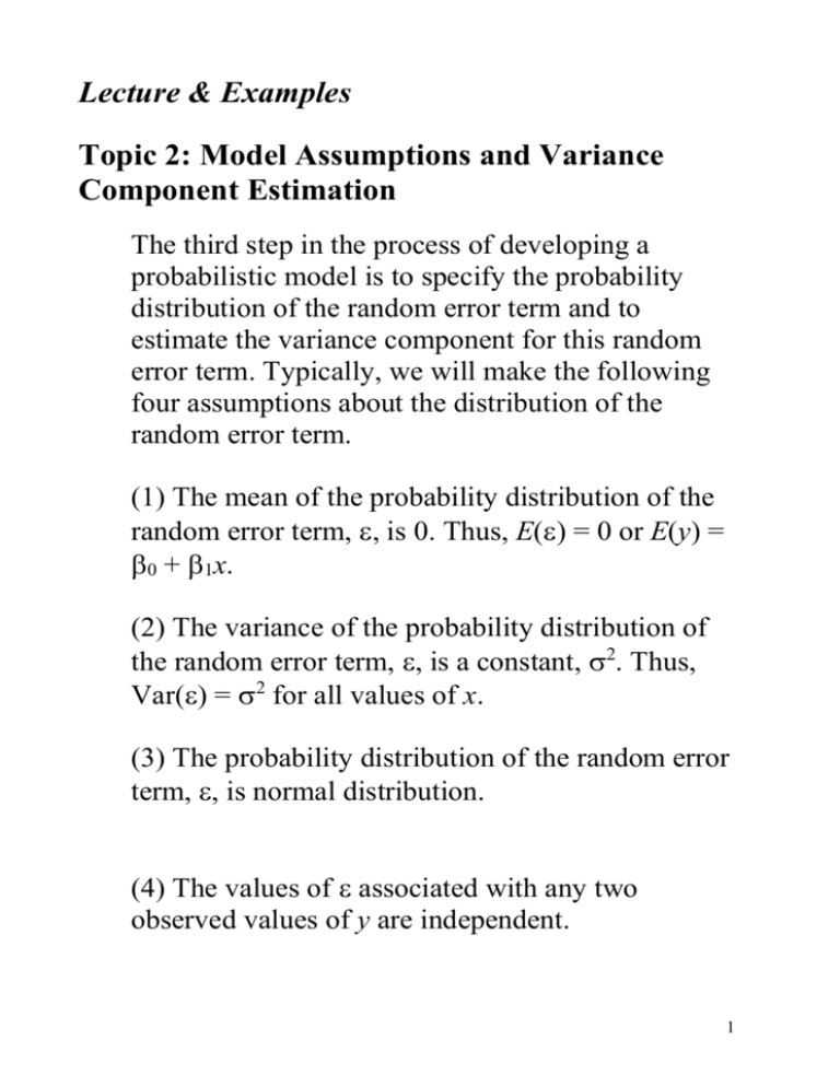
Lecture & Examples
Topic 2: Model Assumptions and Variance
Component Estimation
The third step in the process of developing a
probabilistic model is to specify the probability
distribution of the random error term and to
estimate the variance component for this random
error term. Typically, we will make the following
four assumptions about the distribution of the
random error term.
(1) The mean of the probability distribution of the
random error term, , is 0. Thus, E() = 0 or E(y) =
0 + 1x.
(2) The variance of the probability distribution of
the random error term, , is a constant, 2. Thus,
Var() = 2 for all values of x.
(3) The probability distribution of the random error
term, , is normal distribution.
(4) The values of  associated with any two
observed values of y are independent.
1
With these four assumptions, the least-squares
estimates of the parameters discussed in Topic 1
are the best estimates we can get. Although these
assumptions are very difficult to prove, these
assumptions are reasonable in many practical
problems.
Now, we need to discuss how to find a leastsquares estimator for 2. It is not difficult to show
that the least-squares estimator for 2 is s2 = SSE 
(n - 2), where
yi
d


,
2
b g
SSE   yi  yi  SS yy   1SS xy , SS yy   yi2
2
n
and n is the number of observations in the data.
Consequently, the estimate standard
deviation for  is s  s2 . We will provide either
SAS printout or SSE and SSyy in the exam and
practice problems for the whole semester.
2
Example 11.3:
Calculate SSE and s2 for each of the following
cases:
(a) n  20, SS yy  95, SSxy  50, and  1  0.75
Solution:
SSE  SS yy   1SS xy  95  (0.75)(50)  57.5
s2 
SSE
57.5

 319
.
( n  2)
18
 y 2  860,  y  50,
(b) n  40,
SS xy  2,700, and  1  0.2
Solution:
SS yy   y
2
d i

y
n
2
(50) 2
 860 
 797.5
40
SSE  SS yy   1SS xy  797.5  (0.2)(2,700)  257.5
s2 
SSE
257.5

 6.776
( n  2)
38
(c) n  10, SS yy  58, SS xy  91, SS xx  170
Solution:
SS
91
 1  xy 
 0.535
SS xx
170
SSE  SS yy   1SS xy  58  (0.535)(91)  9.288
s2 
SSE
9.288

 1161
.
( n  2)
8
3
Example 11.4:
In a random sample of n = 9 steers, the live weights
and dressed weights were recorded. In the
following table, we let y denote the dressed weight
(in hundreds of pounds) and x denote the
corresponding live weight (in hundreds of pounds).
Live Weight (x)
4.2
3.8
4.8
3.4
4.5
4.6
4.3
3.7
3.9
Dressed Weight (y)
2.8
2.5
3.1
2.1
2.9
2.8
2.6
2.4
2.5
(a) What assumptions do we need to make about
the distribution of the random error term in our
probabilistic model y = 0 + 1x +  ?
Solution:
(1) E() = 0
(2) Var() = 2
(3) The distribution of  is a normal
distribution
(4) The values of  associated with any two
4
observed values of y are independent
(b) We know that SSyy = 0.72, SSxy = 1.06, and SSxx
= 1.72. Compute SSE and s2.
Solution:
SS
106
.
 1  xy 
 0.616
SS xx
172
.
SSE  SS yy   1SS xy  0.72  (0.616)(106
. )  0.06674
s2 
SSE
0.06674

 0.00953
( n  2)
7
5